AN OPTIMAL CONTROL SOLUTION USING
MULTIPLE SHOOTING METHOD
Said Munzir, Vera Halfiani and Marwan
Abstract. This paper concerns with the solution of optimal control. Optimal
control is an optimization model which generally consists of differential equations system, where the system is built on the state variables representing the system’s condition over time and the control variables which is the decision variables to be determined, so the optimal value of the objective criterion is obtained. Optimal control problem mostly has nonlinear system that is difficult to solve analytically. Therefore, the numerical method could be an alternative solution that can be im-plemented to the problem. One of the numerical methods to solve optimal control problem is Multiple Shooting Method. This method is essentially used to solve the Boundary Value Problem (BVP) on the discussion of differential equations. This method will transform the optimal control problem into numerical formulation in Nonlinear Programming (NLP) form. Furthermore, the NLP can be solved by us-ing the Lagrange Multiplier method, so that the nonlinear algebraic system will be obtained. The final solution of the problem is obtained by implementing the Newton Method to the nonlinear equations system. Afterwards, the second order sufficient condition is applied to guarantee that the final solution is the desired optimal solution.
1. INTRODUCTION
Optimal control is a part of dynamic optimization which aims to determine control variables so that an optimal value of the objective function is ob-tained while satisfying some constraints related to the problem system [1].
Received 22-05-2012, Accepted 13-07-2012.
2010 Mathematics Subject Classification: 49J20,
Key words and Phrases: Optimal control, shooting method, Lagrange Multiplier.
Optimal control problem is formulated in the form of differential equations. It consists of state variables which represent condition of the system over time and control variables which is the decision variables to be determined in order to obtain the optimal value of the objective function.
This paper explains the use of multiple shooting method to numerically solve an optimal control problem. The implementation of this method is supported by some other methods. Multiple shooting method is one of nu-merical method which was firstly found to solve optimal control problem. Essentially, this method is used to solve boundary value problem in differ-ential equation scope. Therefore, this method is sufficient to be applied in optimal control problem which consists of differential equations system and often formulated in boundary value problem. By applying multiple shoot-ing method, the system of differential equations will be transformed into numerical formulation.
Multiple shooting will transform an optimal control problem into a non-linear programming problem. The constraints which are differential equa-tions will be turned into a system of ordinary non-linear algebraic equaequa-tions. Subsequently, the non-linear equations constraints and the objective func-tion which are now a problem of non-linear programming are combined using Lagrange Multiplier. Finally, a Lagrangian function that represent the original optimal control problem is obtained. This new function is an optimization problem without any constraints and its optimum values can be determined through finding its first derivative. The first derivative will be in the form of system of non-linear equations and the solution of this system are found using Newton method which is implemented in Matlab language programming.
Newton method will provide a stationary point which optimize the La-grangian function. However, this point can be either the maxima, the minima, or the saddle point. To verify this point, second order sufficient condition is required. If the point do not satisfy the sufficient condition, then the Newton iteration is repeated to produce a new point. Otherwise, the point is the optimum solution to the initial optimal control problem.
2. THEORIES AND METHODS
Formally, optimal control problem consists of a time variable t, state vari-ablesx(t), control varibles u(t), state equations ˙x(t), boundary conditions, and an objective functionJ. Timetis a continous unit and defined in a cer-tain interval with initial time ti and boundary time tf. Generally, optimal control problem is written in to the following system.
min u(t) J =
Z tf
ti
I(x(t),u(t), t)dt+F(x1, t1),
subjects to
˙
x(t) =f(x(t),u(t), t),
x(ti) =xi,
(x(t), t)∈En+1, when t=tf
u(t)∈Er
The objective function of optimal control problem is a mapping from control functions to a real number value which will be maximized or minimized [2].
2.2 Multiple Shooting Method
Shooting method is a method to solve a boundary value problem in differen-tial equations problem. To ilustrate the concept of this method, it is given the following equation.
˙
x(t) =x(t), ti≤t≤tf.
The analytical solution of above equation is x(t) =x(ti)et−ti,
with e= 2.71. Then x(ti) =xi will be determined such that it will satisfy x(tf) =bfor given valueb. Therefore, equationx(tf)−b= 0 orxiet−ti−b=
0 is obtained. This derivation is called as shooting method. Generally, the shooting method can be summarized as follow.
• Give an initial value xi =x(ti).
In multiple shooting method, the ”shoot” interval is partitioned into some short intervals. It is given the system of differential equations below.
˙
x(t) =f(x(t), t), ti< t < tf. (1) The initial values xi=x(ti) are then determined such that the boundary value
ϕ(x(tf), tf) =0
will give values that satisfy equation (1). The idea of multiple shooting method is splitting the time domaintinto some shorter intervals. letxk for k= 0,1,2, ..., m−1 be the initial value for the dynamic variables at starting point of every short interval segment k+ 1. At each segment k+ 1, the solution of the differential equations from tk totk+1 is established, and let
the solution bexbk. From every interval segment, it can be defined the set of non-linear programming variables as (x0,x1, ...,xm−1). To ensure that the
solution function at each segment forms a single continuous function, the following constraint is formed [3].
[x1−xb0,x2−xb1, ..., ϕ(x(tm), tm)] =0.
2.3 Euler Method
To implement the multiple shooting method, a solution equation of the state equation is needed. The solution can be found either analytically or numerically. However, there is always a case in the initial value problem that the analytical solution can not be determined. Hence, Euler method can be used to form the approximate solution. Let
˙
x(t) =f(t, x) x(ti) =xi ti ≤t≤tf
The interval [ti, tf] is divided intomsubintervals that are bounded by mesh pointtk =ti+k∆tfork= 1,2, . . . , mwhere ∆t= (tf−ti)/mand then the approximate valuex0, x1, . . . , xmofx(t0), x(t1), . . . , x(tm) is determined [4]. The parameter ∆tis called step size [5].
The gradient at (t0, x0) is f(t0, x0) where x0 is the initial condition which
is given. Hence, the tangent line which passes point (t0, x0) is x −x0 =
s(t0, x0)(t−t0) [6]. Generally, the equation used in Euler method can be
written as follow.
.
2.4 Lagrange Multiplier
Lagrange multiplier method is a formulation to get a solution of optimization problem with constraints. Using this method, a non-linear optimization is transformed into a new function with new additional variables, this function is called as Lagrangian. Lagrangian is defined as the sum of an objective function and the linear combination of its constraints [7].
Letz∗ is the local minimizer of a functionf which has constraintsh(z) = 0
and assume that the gradients of the constraints which are∇h1(z∗), . . . ,∇hm(z∗)
are linearly independent. There is a unique vectorλ∗ = [λ∗
1, . . . , λ∗m] which is called Lagrange multiplier such that
∇f(z∗) +
m
X
i=1
λ∗
i∇hi(z∗) = 0
[8].
The Lagrangian can be defined as
L(z,λ) =f(z) +λTh(z)
with necessary condition
∇zL(z,λ) =0 (2) ∇λL(z,λ) =0 (3) [9].
2.4.1 First Order Necessary Condition
From the derivation of Lagrange multiplier method, it can be conclude the first order necessary condition as follow [9].
Theorem 1 Let z∗ be the local extreme value of a function f whose con-straintsh(z) = 0and assume thatz∗ is the regular point of the constraints, then there exists λ∈Em such that
2.4.2 Second Order Condition
Equation (2) and (3) define the necessary condition of the Lagrange mul-tiplier method where the solution of the equations can give the maximum value as well. The second order condition provides the following two things [11].
a. A condition which a point should satisfy in order to be local minimizer (necessary condition)
b. A condition which ensure that the point is the local minimizers (suf-ficient condition)
Second order conditions are stated as follow [9].
Theorem 2 (Second order necessary condition) Letz∗be the local min-imizer of a function f whose constraintsh(z) = 0andz∗ is a regular point of the constraints, then there exists λ∈Em such that
∇f(z∗) +λT∇h(z∗) = 0.
If M ={v|∇h(z∗)v = 0} is the tangent plane, then matrix
∇zzL(z∗) =∇zzf(z∗) +λT∇zz(h(z∗)
is positive semidefinite on M, which isvT∇zzL(z∗)v≥0for every v∈M.
Theorem 3 (Second order sufficient condition) If there exists a point z∗ that satisfies h(z∗) = 0 andλ∈Em such that
∇f(z∗) +λT∇h(z∗) = 0, and matrix
∇zzL(z∗) =∇zzf(z∗) +λT∇zz(h(z∗)
is positive definite on M ={v|∇h(z∗)v = 0}, which is that for every v ∈
M,v 6=0, it applies vT∇zzL(z∗)v>0, thenz∗ is the strict local minimizer
of the function f with constraintsh(z∗) = 0.
The symbol ∇zzf(z) represents the Hessian matrix of the function f with respect to z, that is a m ×m matrix, ∇zzf(z) = [akl] =
h∂2f(z)
∂zk∂zl
i
2.4.3 Some Properties of Matrix
The determination of the properties of matrix ∇zzL(z) (positive/negative definite or semidefinite, or indefinite) in the Theorem 3 will determine the type of extreme pointz∗. Therefore, some explanation about this properties
is necessary. Let A be a symmetrical matrix, then A is positive definite if and only if
wTAw >0
for every non-zero vector w. However, this property is not always easy to be determined. There is another simple equivalent property which involves the eigen values of matrixA. A matrixAmay have the following properties [10].
a. Positive definite, if wTAw >0 for every w or if all the eigen values of Aare positive.
b. Positive semidefinite, if wTAw≥0 for every w or if all the eigen values ofA are non-negative.
c. Negative definite, ifwTAw < 0for everyw or if all the eigen values of Aare negative.
d. Negative semidefinite, if wTAw≤0 for every w or if all the eigen values ofA are non-positive.
e. Indefinite, ifwTAwis both positive and negative or if all eigen values of Aare both positive and negative.
Another approach to determine these properties of a symmetrical matrix is to find the determinant of its leading principal minor [11].
Theorem 4 (Properties of a symmetrical matrix) It is given that a symmetrical m×m matrix A, the following hold.
a. If A is positive semidefinite or positive definite then det(A) ≥ 0 or
det(A)>0 respectively.
b. A is positive definite if and only if all its leading principal minors are positive, that is Ak >0 for k= 1,2, . . . , m.
d. A is negative definite if and only if all the leading principal minors of
−A are positive, that is −Ak>0 for k= 1,2, . . . , m.
e. A is negative semidefinite if and only if all the principal minors of
−A are non-negative, that is −A(kq) ≥ 0 for all possible selection of
{q1, q2, . . . , qk} for k= 1,2, . . . , m.
f. A is indefinite if (c) and (e) are not satisfied.
2.5 Newton Method
Newton method can be used to find the root of an equation. This method uses iteration and requires the guessed initial value for the roots. The for-mula used in this iteration requires the first derivative of the function of the equation,
b
z=z0−
f(z0)
f′(z0) (4)
where z0 is the guessed initial value, and zbis the root of the function f(z)
[12].
In multi-variables equations system, the the formula used in Newton itera-tion is similar to the equaitera-tion (4). For instance, it will be determined the l−vectorz= (z1, . . . , zl) such that
It is assume that the number of functions is the same as the number of varables, m=l. Hence, the linear approach of newton method is
f(bz) =f(z) +G(zb−z) whereGis Jacobian matrix which is defined as
Applying f(zb) = 0 gives the following linear system
Gp=−f(z) (5)
After findingpfrom the equation (5), the solutionzbis determined by looping the following equation
b
z =z+p
To solve the equation (5), it is important to make sure that the Jacobian G is a non-singular matrix. This is the same condition to the problem a function with a single variable in equation (4) where f′(z)6= 0 [3].
2.6 MATLAB
MATLAB (stands for MATrix LABoratory) is a computer software which is developed by Math Works Inc. This software has beed widely used in many fields such as sciences and engineering. MATLAB is a programming language with interactive environment to develop algorithm, data visual-ization, data analysis, and numerical calculation. MATLAB can solve the technical calculation problem faster compared to other traditional language programming software such as C, C++, and Fortran [13].
With its optimal calculation in processing matrices and vectors, MATLAB can provide intuitive language to express problems and their solutions math-ematically or visually. MATLAB is used for various purposes, some of them are stated as follow [14].
a. Developing algorithm ans numerical calculation. b. Symbolic calculation.
c. Modelling, Simulations, and prototype development. d. Data analysis and image processing.
e. Science and engineering visualization.
3. RESULT
It is given the following optimal control problem.
minJ =
Z tf
ti
I(x(t), u(t), t)dt, (6)
subjects to
˙
x(t) =f(x(t), u(t), t), (7)
x(tf) =xf, (8)
(x(t), t)∈R2, (9)
u(t)∈R (10)
The state equation (7) is an ordinary differential equation with boundary condition (8). By implementing multiple shooting method, the domain in-tervaltis partitioned into some subintervals. Let
ti=t0< t1 < . . . < tm =tf.
then, the solution of state equation (7) is determined at every subinterval [tk, tk+1 fork= 0,1,2, . . . , m−1.
For k = 0,1,2, . . . , m−1, let x(tk) = xk be the given initial value for the state equation’s solution andu(tk) =uk at every interval [tk, tk+1].By using
Euler method, the value x(tk+1) is obtained as the following formulation.
x(tk+1)=xk+ ∆tk+1f(xk, uk, tk) where ∆tk+1=tk+1−tk.
The above equation is the solution of the state equation whose value will be found at every subinterval simultaneously. However, to make the final solution function continuous at interval [ti, tf], it is defined that the initial value xk+1 at every subinterval is the same as the boundary value x(tk+1)
at the preceding subinterval.
x(tk+1) =xk+1
x(tk+1)−xk+1= 0
xk+ ∆tk+1f(xk, uk, tk)−xk+1= 0
- (10) is obtained.
The above optimization system is now a constrained non-linear program-ming problem which can be solve by applying Lagrange multiplier method.
Let λ = (λ1, λ2, . . . , λm) be a vector of the Lagrange multiplier, then the
previous constrained non-linear programming system can be reformulated as follow.
and the first order condition are
∇xL(x,u,λ) =0 (11) ∇yL(x,u,λ) =0 (12) ∇λL(x,u,λ) =0 (13) wherex= (x0, x1, . . . , xm) and u= (u0, u1, . . . , um−1).
To see how the Newton method which is implemented in a code program works to this problem, it is given the example below.
minJ =
Z 1
0
x2+u2dt, (14)
subjects to
˙
x(t) = (x−tu)2 (15)
x(1) = 2,(x(t), t)∈R2 (16)
u(t)∈R (17)
Here, the domain interval tis divided into four partitions by step size ∆t= 0.25. Hence, the optimal control problem (14) - (17) can be transformed into the system below.
minJ =
3 X
k=0
(x2k+u2k)0.25 (18)
subject to
x0+ 0.25x20−x1= 0 (19)
x1+ 0.25(x1−0.25u1)2−x2= 0 (20)
x2+ 0.25(x2−0.5u2)2−x3= 0 (21)
x3+ 0.25(x3−0.75u3)2−2 = 0 (22)
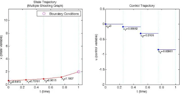
By setting initial value 10 to every variable x, u, λ in Newton iteration implementation, The solutions are found at sixth iteration. The solution list below is produced by the code program implemented using Matlab.
x0= 0.64720, u0 = 0.00000, λ1 =−0.24448
x1= 0.75191, u1 =−0.08652, λ2=−0.044740
x2= 0.90150, u2 =−0.31050, λ3=−0.58765
x3= 1.18069, u3 =−0.83951, λ4=−0.61832
with objective function valueJ =P3k=0(x2k+u2k)0.25 = 0.99991.
the Lagrangian of the optimization system (18) - (22) that is bounded by the null space of the first derivative of constraints (19) - (22). The result shows that the eigen values{0.4308,0.6716,0.4944,0.5000} and the leading principal minor A1 = 0.50000, A2 = 0.24619, A3 = 0.11450, A4 = 0.05023
Figure 1: State Trajectory and Control Trajectory of Optimal Control Problem (14) - (17) at Iteration 1 - 6
3.2 Linear Optimal Control Problem and The guessed Initial Value for Newton Iteration
To solve the constrained non-linear programming formulation by using La-grange multiplier, the objective function and the constraints have to be twice differentiable. In other words, if the system is linear onxanduthen matrix ∇zzL(z) =0 (wherez= (x, u)) on all the domain points causing the local minimizer can not be determined. If the first order conditions (11) - (13) are satisfied but the Hessian matrix of the Lagrangian which is the second order condition is zero (or the determinant is zero), then the point that satisfies this condition is called singular point. Moreover, the final solution using Newton method requires the first derivative (the Jacobian matrix) of the system (11) - (13). This derivative is equivalent to the second deriva-tive (the Hessian matrix) of the LagrangianLwith respect tox, u, λ. This matrix has to be invertible or a non-singular matrix so that the Newton iteration can work. This condition constrains that the Lagrangian has to be twice differentiable.
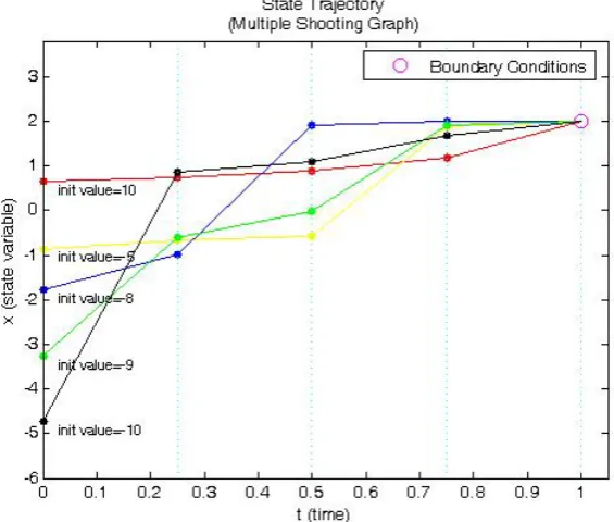
minimizer. Meanwhile, initial values −2 and −4 cause the iteration never ends and does not give any solution point. The graphs of the state variable for various guessed initial value are represented in Figure 2. The red line represents the state variable which is obtained from the final solution by giving the initial value 10 in the Newton iteration, while the yellow, blue, green, and black line (which is not the solution) represents the state variable which is obtained by setting the initial values−5,−8,−9,−10 respectively.
Figure 2: State Trajectory of Optimal Control Problem (14) - (17) obtained from some different initial values setting
4. CONCLUSION AND FUTURE RECOMMENDATION
4.1 Conclusion
a. By using multiple shooting method, an optimal control problem can be transformed into a numerical formulation in constrained non-linear programming form which can be solved by using Lagrange multiplier method.
c. The solution obtained from the Newton method can be either maxi-mum, minimaxi-mum, or saddle point. Therefore, the second order condi-tion is required to confirm that the solucondi-tion point is the appropriate extreme point to the original problem.
4.2 Future Recommendation
a. In this study, the optimal control problem that is implemented consists of one state and control variable. The future study may consider the problem with multi variables.
b. The step size of the domain interval can be made smaller so that the more accurate solution can be obtained.
c. The code program in this study is only the implementation of Newton method. The future study may consider to code the whole methods used.
REFERENCES
1. Kirk, Donald E, Optimal Control Theory, An Introduction, Dover Publica-tions Inc., New York, 1970.
2. Intriligator, Michael D, Mathematical Optimization and Economics The-ory, Society for Industrial and Applied Mathematics, Philadelphia, 2001. 3. Betts, John T.,Practical Methods for Optimal Control Using Non-linear
Pro-gramming, Society for Industrial and Applied Mathematics, Philadelphia, 2001. 4. Dahlquist, Germund, and ˚Ake Bj¨orck, Ned Anderson,Numerical
Meth-ods, Dover Publication, Inc., New York, 1974.
5. Mathews, John H. dan Kurtis D. Fink, Numerical Methods Using MAT-LAB, Third Edition, Prentice Hall. USA, 1999.
6. Buchanan, James L. and Peter R. Turner,Numerical Method and Anal-ysis, McGraw-Hill,Inc.,Singapore, 1992.
7. Venkataraman, P,Applied Optimization with MATLAB Programming, A Wiley-Interscience Publication, New York, 2002.
9. Luenberger, David G, Linear and Nonlinear Programming, Springer, New York, 2008.
10. Griva, Igor, dan Stephen G. Nash, Ariela Sofer, Linear and Nonlinear Optimization, Second Edition, Society for Industrial and Applied Mathematics. USA, 2009.
11. Antoniou, Andreas and Wu-Sheng Lu,Practical Optimization; Algorithms and Engineering Applications, Springer, New York, 2007.
12. Daniels, Richard W,An Introduction to Numerical Methods and Optimization Techniques, Elsevier North-Holland. New York, 1978.
13. The MathWorksTM, MATLABr Getting Started Guide, The MathWorks, Inc., United States, 2010.
14. Dukkipati, Rao V, MATLAB An Introduction With Applications, New Age International (P) Ltd., Publishers, New Delhi, 2010.
Said Munzir: Jurusan Matematika, FMIPA, Universitas Syiah Kuala, Jl. Tgk. Daud Beureuh No. 4 Darussalam-Banda Aceh 23111, Indonesia.
E-mail: [email protected]
Vera Halfiani: Jurusan Matematika, FMIPA, Universitas Syiah Kuala, Jl. Tgk. Daud Beureuh No. 4 Darussalam-Banda Aceh 23111,Indonesia.