Learning the Information Divergence

(1)

Learning the Information Divergence

Onur Dikmen,

Member, IEEE,

Zhirong Yang,

Member, IEEE,

and Erkki Oja,

Fellow, IEEE,

Abstract—Information divergence that measures the difference between two nonnegative matrices or tensors has found its use in a variety of machine learning problems. Examples are Nonnegative Matrix/Tensor Factorization, Stochastic Neighbor Embedding, topic models, and Bayesian network optimization. The success of such a learning task depends heavily on a suitable divergence. A large variety of divergences have been suggested and analyzed, but very few results are available for an objective choice of the optimal divergence for a given task. Here we present a framework that facilitates automatic selection of the best divergence among a given family, based on standard maximum likelihood estimation. We first propose an approxi-mated Tweedie distribution for theβ-divergence family. Selecting the best β then becomes a machine learning problem solved by maximum likelihood. Next, we reformulate α-divergence in terms of β-divergence, which enables automatic selection of α

by maximum likelihood with reuse of the learning principle for

β-divergence. Furthermore, we show the connections betweenγ -and β-divergences as well as Rényi- and α-divergences, such that our automatic selection framework is extended to non-separable divergences. Experiments on both synthetic and real-world data demonstrate that our method can quite accurately select information divergence across different learning problems and various divergence families.

Index Terms—information divergence, Tweedie distribution, maximum likelihood, nonnegative matrix factorization, stochastic neighbor embedding.

I. INTRODUCTION

Information divergences are an essential element in modern machine learning. They originated in estimation theory where a divergence maps the dissimilarity between two probability distributions to nonnegative values. Presently, information divergences have been extended for nonnegative tensors and used in many learning problems where the objective is to min-imize the approximation error between the observed data and the model. Typical applications include Nonnegative Matrix Factorization (see e.g. [1], [2], [3], [4]), Stochastic Neighbor Embedding [5], [6], topic models [7], [8], and Bayesian network optimization [9].

There exist a large variety of information divergences. In Section II, we summarize the most popularly used parametric families includingα-,β-,γ- and Rényi-divergences [10], [11], [12], [13], [14] and their combinations (e.g. [15]). The four parametric families in turn belong to broader ones such as

the Csiszár-Morimoto f-divergences [16], [17] and Bregman

divergences [18]. Data analysis techniques based on informa-tion divergences have been widely and successfully applied to various data such as text [19], electroencephalography [3], facial images [20], and audio spectrograms [21].

The authors are with Department of Information and Computer Sci-ence, Aalto University, 00076, Finland. e-mail: onur.dikmen@aalto.fi; zhi-rong.yang@aalto.fi; erkki.oja@aalto.fi

Compared to the rich set of available information diver-gences, there is little research on how to select the best one for a given application. This is an important issue because the performance of a given divergence-based estimation or modeling method in a particular task very much depends on the divergence used. Formulating a learning task in a family of divergences greatly increases the flexibility to handle different types of noise in data. For example, Euclidean distance is suitable for data with Gaussian noise; Kullback-Leibler diver-gence has shown success for finding topics in text documents [7]; and Itakura-Saito divergence has proven to be suitable for audio signal processing [21]. A conventional workaround is to select among a finite number of candidate divergences using a validation set. This however cannot be applied to divergences that are non-separable over tensor entries. The validation approach is also problematic for tasks where all data are needed for learning, for example, cluster analysis.

In Section III, we propose a new method of statistical learning for selecting the best divergence among the four popular parametric families in any given data modeling task. Our starting-point is the Tweedie distribution [22], which is known to have a relationship with β-divergence [23], [24]. The Maximum Tweedie Likelihood (MTL) is in principle a disciplined and straightforward method for choosing the optimalβ value. However, in order for this to be feasible in practice, two shortcomings with the MTL method have to be overcome: 1) Tweedie distribution is not defined for all β; 2) calculation of Tweedie likelihood is complicated and prone to numerical problems for largeβ. To overcome these drawbacks, we propose here a novel distribution using an exponential over theβ-divergence with a specific augmentation term. The new distribution has the following nice properties: 1) it is close to the Tweedie distribution, especially at four important special cases; 2) it exists for allβ ∈R; 3) its likelihood can be calcu-lated by standard statistical software. We call the new density the Exponential Divergence with Augmentation (EDA). EDA is a non-normalized density, i.e., its likelihood includes a normalizing constant which is not analytically available. But, since the density is univariate the normalizing constant can be efficiently and accurately estimated by numerical integration. The method of Maximizing the Exponential Divergence with Augmentation Likelihood (MEDAL) thus gives a more robust

β selection in a wider range than MTL.β estimation on EDA

can also be carried out using parameter estimation methods, e.g., Score Matching (SM) [25], specifically proposed for non-normalized densities. In the experiments section, we show that SM on EDA also performs as accurately as MEDAL.

Besides β-divergence, the MEDAL method is extended to

select the best divergence in other parametric families. We reformulate α-divergence in terms of β-divergence after a

(2)

MEDAL method. Our method can also be applied to

non-separable cases. We show the equivalence between β and

γ-divergences, and between α and Rényi divergences by a

connecting scalar, which allows us to choose the best γ- or Rényi-divergence by reusing the MEDAL method.

We tested our method with extensive experiments, whose re-sults are presented in Section IV. We have used both synthetic data with a known distribution and real-world data including music, stock prices, and social networks. The MEDAL method is applied to different learning problems: Nonnegative Matrix Factorization (NMF) [26], [3], [1], Projective NMF [27], [28] and Symmetric Stochastic Neighbor Embedding for visualiza-tion [5], [6]. We also demonstrate that our method outperforms Score Matching on Exponential Divergence distribution (ED), a previous approach for β-divergence selection [29]. Conclu-sions and discusConclu-sions on future work are given in Section V.

II. INFORMATIONDIVERGENCES

Many learning objectives can be formulated as an approxi-mation of the form x_≈µ, where x>0 is the observed data

(input) and µ is the approximation given by the model. The

formulation for µ totally depends on the task to be solved. Consider Nonnegative Matrix Factorization: then x >0 is a data matrix andµis a product of two lower-rank nonnegative matrices which typically give a sparse representation for the

columns of x. Other concrete examples are given in Section

IV.

The approximation error can be measured by various

in-formation divergences. Suppose µ is parameterized by Θ.

The learning problem becomes an optimization procedure that minimizes the given divergence D(x_||µ(Θ)) over Θ. Regularization may be applied for Θ for complexity control. For notational brevity we focus on definitions over vectorialx, µ,Θ in this section, while they can be extended to matrices or higher order tensors in a straightforward manner.

In this work we consider four parametric families of di-vergences, which are the widely used α-,β-,γ- and Rényi-divergences. This collection is rich because it covers most commonly used divergences. The definition of the four fami-lies and some of their special cases are given below.

• α-divergence [10], [11] is defined as

Dα(x_||µ) = P

ixαiµ1i−α−αxi+ (α−1)µi

α(α−1) . (1)

The family contains the following special cases:

Dα=2(x_||µ) =DP(x||µ) =1

Kullback-Leibler, Pearson Chi-square, inverse Pearson and Hellinger distances, respectively.

• β-divergence [30], [31] is defined as

Dβ(x_||µ) =

The family contains the following special cases:

Dβ=1(x_||µ) =DEU(x||µ) = 1

whereDEU andDIS denote the Euclidean distance and

Itakura-Saito divergence, respectively. • γ-divergence [13] is defined as

Dγ(x||µ) = 1

The normalized Kullback-Leibler (KL) divergence is a special case ofγ-divergence:

Dγ→0(x||µ) =DKL(˜x||µ˜) =

• Rényi divergence [32] is defined as

Dρ(x_||µ) = 1

for ρ > 0. The Rényi divergence also includes the normalized Kullback-Leibler divergence as its special case when ρ_→1.

III. DIVERGENCESELECTION BYSTATISTICALLEARNING

The above rich collection of information divergences basi-cally allows great flexibility to the approximation framework.

However, practitioners must face a choice problem: how to

select the best divergence in a family? In most existing applications the selection is done empirically by the human. A conventional automatic selection method is cross-validation [33], [34], where the training only uses part of the entries

of x and the remaining ones are used for validation. This

(3)

Second, separation of some entries is not applicable in applica-tions where all entries are needed in the learning, for example, cluster analysis. Third, cross-validation errors defined with dif-ferent divergences are not comparable because the comparison has no statistical meaning. Fourth, quantifying cross-validation errors by Dβ(x_||µ)often selects β with the largest absolute values. Letxiandµithe validation entries. For anyxi∈(0,1)

and µi ∈ (0,1), we have limβ→+∞Dβ(xi||µi) = 0 by

l’Hôpital’s rule. That is, the selection in this case does not respect the data at all, but trivially picks the largest candidate

(i.e. +∞). We demonstrate such failure in Section IV-C3.

Similarly, the selection is also problematic for any xi > 1

andµi>1, wherelimβ→−∞Dβ(x||µ) = 0.

Our proposal here is to use the familiar and proven

tech-nique of maximum likelihood estimation for automatic

di-vergence selection, using a suitably chosen and very flexible probability density model for the data. In the following we discuss this statistical learning approach for automatic diver-gence selection in the family of β-divergences, followed by its extensions to the other divergence families.

A. Selecting β-divergence

1) Maximum Tweedie Likelihood (MTL): We start from the probability density function (pdf) of an exponential dispersion model (EDM) [22]:

where φ > 0 is the dispersion parameter, θ is the canonical parameter, andκ(θ)is the cumulant function (whenφ= 1its derivatives w.r.t.θgive the cumulants). Such a distribution has meanµ=κ′₍_θ₎_{and variance}_V₍_{µ, p}_{) =}_φκ′′₍_θ₎_{. This density} is defined for x_≥0, thus µ >0.

A Tweedie distribution is an EDM whose variance has a special form, V(µ) = µp _with _p

∈ R\(0,1). The canonical parameter and the cumulant function that satisfy this property are [22] forms of f(x, φ, p) in Tweedie distribution are generally unavailable. The function can be expanded with infinite series [35] or approximated by saddle point estimation [36].

It is known that the Tweedie distribution has a connection to β-divergence (see, e.g., [23], [24]): maximizing the likelihood of Tweedie distribution for certain p values is equivalent to minimizing the corresponding divergence withβ= 1₋p. Es-pecially, the gradients of the log-likelihood of Gamma, Poisson and Gaussian distributions overµi are equal to the ones ofβ

-divergence withβ =₋1,0,1, respectively. This motivates aβ -divergence selection method by Maximum Tweedie Likelihood (MTL).

However, MTL has the following two shortcomings. First, Tweedie distribution is not defined for p∈(0,1). That is, if the bestβ= 1−phappens to be in the range(0,1), it cannot

be found by MTL; in addition, there is little research on the Tweedie distribution with β >1 (p < 0). Second, f(x, φ, p)

in Tweedie distribution is not the probability normalizing constant (note that it depends onx), and its evaluation requires ad hoc techniques. The existing software using the infinite series expansion approach [35] (see Appendix A) is prone to numerical computation problems especially for₋0.1< β <0. There is no existing implementation that can calculate Tweedie likelihood forβ >1.

2) Maximum Exponential Divergence with Augmentation Likelihood (MEDAL): Our answer to the above shortcomings in MTL is to design an alternative distribution with the following properties: 1) it is close to the Tweedie distribution, especially for the four crucial points whenβ∈ {−2,−1,0,1}; 2) it should be defined for allβ ∈R; 3) its pdf can be evaluated more robustly by standard statistical software.

From (10) and (11) the pdf of the Tweedie distribution is written as

To make an explicit connection with β-divergence defined in (2), we suggest a new distribution given in the following form:

Now theβ-divergence for scalarxappears in the exponent, and g(x, φ, β) will be used to approximate this with the Tweedie distribution. Ideally, the choice

g(x, φ, β) =f(x, φ, β)/exp

would result in full equivalence to Tweedie distribution, as seen from (12). However, because f(x, φ, β) is unknown in the general case, suchg is also unavailable.

We can, however, try to approximateg using the fact that papproxmust be a proper density whose integral is equal to one.

From (13) it then follows

(4)

wherex0= arg maxxh(x)andM is a large constant.

In order to approximate (14) by Laplace’s method, 1/φ

takes the role of M and thus the approximation is valid for

small φ. We need the maximizer of the exponentiated term

h(x) =₋ xβ+1

β(β+1)+ xµβ

β . This term has a zero first derivative

and negative second derivative, i.e., it is maximized, atx=µ. Thus, Laplace’s method gives us

exp

Putting this result into (13) as such does not guarantee a proper pdf however, because it is an approximation, only valid

at the limit φ _→ 0. To make it proper, we have to add a

normalizing constant into the density in (13).

The pdf of the final distribution, for a scalar argument x, thus becomes

where Z(µ, β, φ) is the normalizing constant counting for the terms which are independent of x, and R(x, β) is an augmentation term given as

R(x, β) = β−1

2 lnx . (16)

This pdf is a proper density for all β ∈ R, which is

guaranteed by the following theorem.

Theorem 1: Let f(x) = expnβ−₂1lnx₋1

Finally, for vectorialx, the pdf is a product of the marginal densities:

We call (17) the Exponential Divergence with Augmentation (EDA) distribution, because it applies an exponential over an information divergence plus an augmentation term.

The log-likelihood of the EDA density can be written as

lnp(x;µ, β, φ) =X term in (18) are separable over xi, (i.e. xi are independent

givenµi). The bestβ is now selected by

selection methodMaximum EDA Likelihood (MEDAL).

Let us look at the four special cases of Tweedie distribu-tion: Gaussian (_N), Poisson (_PO), Gamma (_G) and Inverse Gaussian (_IN). They correspond to β = 1,0,₋1,₋2. For simplicity of notation, we may drop the subscriptiand write xandµ for one entry in x andµ. Then, the log-likelihoods of the above four special cases are

lnpN(x;µ, φ) =−1₂ln(2πφ)−₂1_φ(x−µ)2,

where in the Poisson case we employ Stirling’s approxima-tion1_{. To see the similarity of these four special cases with the}

general expression for the EDA log-likelihood in Eq. (19), let us look at one term in the sum there. It is a fairly straightforward exercise to plug in the β-divergences from Eqs. (3,4,5,6) and the augmentation term from Eq. (18) and see that the log-likelihoods coincide. The normalizing term

lnZ(µ, β, φ)] for these special cases can be determined from the corresponding density.

In general, the normalizing constant Z(µ, β, φ) is in-tractable except for a few special cases. Numerical evaluation of Z(µ, β, φ) can be implemented by standard statistical software. Here we employ the approximation with Gauss-Laguerre quadratures (details in Appendix B).

Finally, let us note that in addition to the maximum likeli-hood estimator, Score Matching (SM) [25], [37] can be applied

1_{The case}_β_{= 0}_and_φ₆_{= 1}_{does not correspond to Poisson distribution,} but the transformationpEDM(x;µ, φ,1) =pP O(x/φ;µ/φ)/φcan be used

(5)

to estimation ofβas a density parameter (see Section IV-A). In a previous effort, Lu et al. [29] proposed a similar exponential divergence (ED) distribution

pED(x;µ, β)∝exp [−Dβ(x||µ)], (21)

but without the augmentation. It is easy to show that ED also exists for allβby changingq= 1 +ǫin the proof of Theorem 1. We will empirically illustrate the discrepancy between ED and EDA in Section IV-A, showing that the selection based on ED is however inaccurate, especially for β_≤0.

B. Selecting α-divergence

We extend the MEDAL method to α-divergence selection.

This is done by relating α-divergence toβ-divergence with a nonlinear transformation betweenαandβ. Letyi=xαi/α2α,

mi=µαi/α2α andβ= 1/α−1for α6= 0. We have

Dβ(yi||mi) = 1

β(β+ 1)

yβ+1_i +βmβ+1_i ₋(β+ 1)yimβi

=−α 2

α₋1

xi

α2 + 1₋α

α µi

α2 − 1

α xα

i

α2α

µ1_i−α α2(1−α)

=Dα(xi||µi)

This relationship allows us to evaluate the likelihood of µ andαusing yi andβ:

p(xi;µi, α, φ) =p(yi;mi, β, φ)

dyi

dxi

=p(yi;mi, β, φ)

xα_i−1 α2(α−1/2) =p(yi;mi, β, φ)yi−β|β+ 1|

In vectorial form, the best α for Dα(x_||µ) is then given by α∗_{= 1}_/₍_β∗_{+ 1)}_where

β∗= arg max β

n

max φ

lnp(y;m, β)

−βlnyi+ ln|β+ 1|o, (22)

where m= arg minηDβ(y||η). This transformation method

can handle allαexceptα_→0since it corresponds toβ_{→ ∞}. It is important to notice that in our method the transforma-tion takes place not only from αto β, but also from x toy and fromµ tom. Therefore the selectedβ fory andmis in general not the same with the one for xandµ.

C. Selecting γ- and Rényi divergences

Above we presented the selection methods for two families where the divergence is separable over the tensor entries. Next we consider selection amongγ- and Rényi divergence families where their members are not separable. Our strategy is to reduceγ-divergence toβ-divergence with aconnecting scalar. This is formally given by the following result.

Theorem 2: Forx_≥0andτ _∈R,

arg min

µ≥0Dγ→τ(x||µ) = arg minµ≥0

min

c>0Dβ→τ(x||cµ)

(23)

The proof is done by zeroing the derivative right hand side with respect to c(details in Appendix C).

Theorem 2 states that with a positive scalar, the learning

problem formulated by a γ-divergence is equivalent to the

one by the correspondingβ-divergence. The latter is separable and can be solved by the methods described in the Section III-A. An example is between normalized KL-divergence (in γ-divergence) and the non-normalized KL-divergence (in β -divergence) with the optimal connecting scalar c = P_Pixi

iµi. Example applications on selecting the best γ-divergence are given in Section IV-C.

Similarly, we can also reduce a Rényi divergence to its

corresponding α-divergence with the same proof technique

(see Appendix C).

Theorem 3: Forx_≥0andτ >0,

arg min µ≥0Dρ→τ(

x_||µ) = arg min

µ≥0

min

c>0Dα→τ(x||cµ)

. (24)

IV. EXPERIMENTS

In this section we demonstrate the proposed method on various data types and learning tasks. First we provide the results on synthetic data, whose density is known, to compare the behavior of MTL, MEDAL and the score matching method [29]. Second, we illustrate the advantage of the EDA density over ED. Third, we apply our method onα- andβ-divergence selection in Nonnegative Matrix Factorization (NMF) on real-world data including music and stock prices. Fourth, we test MEDAL in selecting non-separable cases (e.g.γ-divergence) for Projective NMF and s-SNE visualization learning tasks across synthetic data, images, and a dolphin social network.

A. Synthetic data

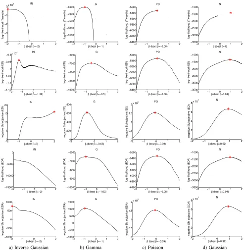
1) β-divergence selection: We use here scalar data gen-erated from the four special cases of Tweedie distributions, namely, Inverse Gaussian, Gamma, Poisson, and Gaussian distributions. We simply fit the best Tweedie, EDA or ED density to the data using either the maximum likelihood method or score matching (SM).

In Fig. 1 (first row), the results of the Maximum Tweedie

Likelihood (MTL) are shown. The β value that maximizes

the likelihood in Tweedie distribution is consistent with the true parameters, i.e., -2, -1, 0 and 1 respectively for the above distributions. Note that Tweedie distributions are not defined forβ_∈(0,1), butβ-divergence is defined in this region, which will lead to discontinuity in the log-likelihood overβ.

The second and third rows in Fig. 1 present results of the exponential divergence density ED given in Eq. (21). The log-likelihood and negative score matching objectives [29] on the same four datasets are shown. The estimates are consistent with the ground truth Gaussian and Poisson data. However, for

Gamma and Inverse Gaussian data, both β estimates deviate

from the ground truth. Thus, estimators based on ED do not give as accurate estimates as the MTL method. The ED distribution [29] has an advantage that it is defined also for β ∈ (0,1). In the above, we have seen that β selection by

using ED is accurate when β → 0 or β = 1. However, as

(6)

−2 −1 0 1 2

negative SM objective (ED)

β (best β=2)

β (best β=−0.63)

β (best β=−0.09)

β (best β=0.92)

negative SM objective (EDA)

β (best β=−2)

β (best β=−1)

β (best β=−0.09)

β (best β=0.92) N

a) Inverse Gaussian b) Gamma c) Poisson d) Gaussian

Fig. 1. βselection using (from top to bottom) Tweedie likelihood, ED likelihood, negative SM objective of ED, EDA likelihood, and negative SM objective of EDA. Data were generated using Tweedie distribution withβ=−2,−1,0,1(from left to right).

the observed variable in these distributions are not exactly the same as those of the Tweedie distributions.

EDA, the augmented ED density introduced in Sec-tion III-A, not only has both the advantage of continuity but also gives very accurate estimates forβ <0. The MEDAL

log-likelihood curves over β based on EDA are given in Fig. 1

(fourth row). In the β selection of Eq. (20), the φ value

that maximizes the likelihood with β fixed is found by a

grid search. The likelihood values are the same as those of special Tweedie distributions and there are no abrupt changes or discontinuities in the likelihood surface. We also estimated

β for the EDA density using Score Matching, and curves of

the negative SM objective are presented in the bottom row of Fig. 1. They also recover the ground truth accurately.

2) α-divergence selection: There is only one known gen-erative model for which the maximum likelihood

estima-tor corresponds to the minimizer of the corresponding α

divergence. It is the Poisson distribution. We thus reused the Poisson-distributed data of the previous experiments with the β-divergence. In Fig. 2a, we present the log-likelihood

objective over α obtained with Tweedie distribution (MTL)

(7)

−2 −1 0 1 2 −3250

−3200 −3150 −3100 −3050 −3000 −2950

log−likelihood (Tweedie)

α (best α=1.01) PO

−2 −1 0 1 2 −3160

−3140 −3120 −3100 −3080 −3060 −3040

log−likelihood (ED)

−2 −1 0 1 2 −3250

−3200 −3150 −3100 −3050 −3000

log−likelihood (EDA)

−21 −1 0 1 2 1.1

1.2 1.3 1.4 1.5 1.6x 10

4

(a) (b) (c) (d)

Fig. 2. Log-likelihood of (a) Tweedie, (b) ED, and (c) EDA distributions forα-selection. In the Tweedie plot, blanks correspond toβ= 1/α−1values for which a Tweedie distribution pdf does not exist or cannot be evaluated, i.e.,β∈(0,1)∪(1,∞). In (d), negative SM objective function values are plotted for EDA.

α → 1 is successfully recovered with MTL. However, there

are no likelihood estimates for α ∈ (0.5,1), corresponding to β_∈(0,1) for which no Tweedie distributions are defined. Moreover, to our knowledge there are no studies concerning the pdf’s of Tweedie distributions withβ >1. For that reason, the likelihood values forα_∈[0,0.5)are left blank in the plot. It can be seen from Fig. 2b and 2c, that the augmentation

in the MEDAL method also helps inαselection. Again, both

ED and EDA solve most of the discontinuity problem except

α = 0. Selection using ED fails to find the ground truth

which equals 1, which is however successfully found by the MEDAL method. SM on EDA recovers the ground truth as well (Fig. 2d).

B. Divergence selection in NMF

The objective in nonnegative matrix factorization (NMF) is to find a low-rank approximation to the observed data by expressing it as a product of two nonnegative matrices,

i.e., V _≈ Vb = WH with V _∈ R+F×N , W ∈ RF+×K

and H _∈ RK+×N. This objective is pursued through the

minimization of an information divergence between the data and the approximation, i.e.,D(V_||Vb). The divergence can be any appropriate one for the data/application such as β, α, γ, Rényi, etc. Here, we chose theβandαdivergences to illustrate the MEDAL method for realistic data.

The optimization of β-NMF was implemented using the

standard multiplicative update rules [23], [38]. Similar mul-tiplicative update rules are also available for α-NMF [23]. Alternatively, the algorithm for β-NMF can be used for α -divergence minimization as well, using the transformation explained in Section III-B.

1) A Short Piano Excerpt: We consider the piano data used in [21]. It is an audio sequence recorded in real conditions, consisting of four notes played all together in the first measure and in all possible pairs in the subsequent measures. A power spectrogram with analysis window of size 46 ms was

computed, leading to F = 513 frequency bins and N = 676

time frames. These make up the data matrix V, for which a

matrix factorizationVb =WHwith low rankK= 6is sought for.

In Fig. 3a and 3b, we show the log-likelihood values of

the MEDAL method for β and α, respectively. For each

parameter valueβ andα, the multiplicative algorithm for the respective divergence is run for 100 iterations and likelihoods

−2 −1 0 1 2

−6 −4 −2 0 2 4x 10

6

β (best β=−1) Piano excerpt

−2 −1 0 1 2

−3 −2 −1 0 1 2x 10

4

α (best α=−0.2) Piano excerpt

a)β div. b) αdiv.

−2 −1 0 1 2

−1 0 1 2 3 4x 10

5

β (best β=−1) Piano excerpt

c)β div.

Fig. 3. (a, b) Log likelihood values forβ and αfor the spectrogram of a short piano excerpt withF = 513,N = 676,K= 6. (c) Negative SM objective forβ.

are evaluated with mean values calculated from the returned matrix factorizations. For each value ofβ andα, the highest likelihood w.r.t.φ(see Eq. (20)) is found by a grid search.

The found maximum likelihood estimate β = ₋1

corre-sponds to Itakura-Saito divergence, which is in harmony with the empirical results presented in [21] and the common belief that IS divergence is most suitable for audio spectrograms. The optimalαvalue value was 0.5 corresponding to Hellinger dis-tance. We can also see that the log likelihood value associated withα= 0.5is still much less than the one for β=₋1. SM also finds β=₋1 as can be seen from Fig. 3c.

2) Stock Prices: Next, we repeat the same experiment on a stock price dataset which contains Dow Jones Industrial Average. There are 30 companies included in the data. They are major American companies from various sectors such as services (e.g., Walmart), consumer goods (e.g., General Motors) and healthcare (e.g., Pfizer). The data was collected from 3rd January 2000 to 27th July 2011, in total 2543 trading

dates. We set K = 5 in NMF and masked 50% of the data

by following [39]. The stock data curves are displayed in

(8)

500 1000 1500 2000 2500 0

50 100 150

days

stock prices

−2 −1 0 1 2

−8 −6 −4 −2

0x 10 4

β (best β=0.4) stock prices

−20 −1 0 1 2 2

4 6 8x 10

8

β (best β=1) stock prices

Fig. 4. Top: thestockdata. Bottom left: the EDA log-likelihood forβ∈

[−2,2]. Bottom right: negative SM objective function forβ∈[−2,2].

The EDA likelihood curve with β _∈ [₋2,2] is shown in Figure 4 (bottom left). We can see that the best divergence

selected by MEDAL is β = 0.4. The corresponding best

φ = 0.006. These results are in harmony with the findings of Tan and Févotte [39] using the remaining 50% of the data as validation set, where they found that β ∈ [0,0.5]

(mind that our β values equal theirs minus one) performs

well for a large range ofφ’s. Differently, our method is more advantageous because we do not need additional criteria nor data for validations. In Figure 4 (bottom right), negative SM objective function is plotted for β _∈ [₋2,2]. With SM, the optimalβ is found to be 1.

C. Selecting γ-divergence

In this section we demonstrate that the proposed method can be applied to applications beyond NMF and to non-separable divergence families. To our knowledge, no other existing methods can handle these two cases.

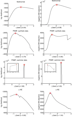
1) Multinomial data: We first exemplify γ-divergence se-lection for synthetic data drawn from a multinomial dis-tribution. We generated a 1000-dimensional stochastic

vec-tor p from the uniform distribution. Next we drew x _∼

Multinomial(n,p) with n = 107_{. The MEDAL method is}

applied to find the best γ-divergence for the approximation of xby p.

Fig. 6 (1st row, left) shows the MEDAL log-likelihood.

The peak appears when γ = 0, which indicates that the

normalized KL-divergence is the most suitable one among the γ-divergence family. Selection using score matching of EDA gives the bestγ also close to zero (Fig. 6 1st row, right). The result is expected, because the maximum likelihood estimator of p in multinomial distribution is equivalent to minimizing

the KL-divergence over p. Our finding also justifies the

usage of KL-divergence in topic models with the multinomial distribution [40], [7].

2) Projective NMF: Next we apply the MEDAL method to Projective Nonnegative Matrix Factorization (PNMF) [27],

[28] based on γ-divergence [13], [19]. Given a nonnegative

matrix V _∈ RF+×N, PNMF seeks a low-rank nonnegative

matrix W _∈ RF+×K (K < F) that minimizes Dγ

V_||Vb,

where Vb = WWTV. PNMF is able to produce a highly

orthogonal W and thus finds its applications in part-based feature extraction and clustering analysis, etc. Different from conventional NMF (or linear NMF) where each factorizing matrix only appears once in the approximation, the matrix Woccurs twice in V. Thus it is a special case of Quadraticb Nonnegative Matrix Factorization (QNMF) [41].

We choose PNMF for two reasons: 1) we demonstrate the MEDAL performance on QNMF besides the linear NMF already shown in Section IV-B; 2) PNMF contains only one variable matrix in learning, without the issue of how to interleave the updates of different variable matrices.

We first tested MEDAL on a synthetic dataset. We generated a diagonal blockwise data matrixVof size50_×30, where two blocks are of sizes30_×20and20_×10. The block entries are uniformly drawn from [0,10]. We then added uniform noise from [0,1]to the all matrix entries. For each γ, we ran the multiplicative algorithm of PNMF by Yang and Oja [28], [4]

to obtainWandV. The MEDAL method was then applied tob

select the bestγ. The resulting approximated log-likelihood for γ_∈[₋2,2]is shown in Fig. 6 (2nd row). We can see MEDAL and score matching of EDA give similar results, where the best γappear at−0.76and−0.8, respectively. Both resultingW’s give perfect clustering accuracy of data rows.

We also tested MEDAL on theswimmerdataset [42] which

is popularly used in the NMF field. Some example images from this dataset are shown in Fig. 5 (left). We vectorized each image in the dataset as a column and concatenated the columns into a1024_×256data matrixV. This matrix is then fed to PNMF and MEDAL as in the case for the synthetic dataset. Here we empirically set the rank toK= 17according

to Tan and Févotte [43] and Yang et al. [44]. The matrix W

was initialized by PNMF based on Euclidean distance to avoid poor local minima. The resulting approximated log-likelihood forγ∈[−1,3]is shown in Figure 6 (3rd row, left). We can see a peak appearing around1.7. Zooming in the region near the peak shows the best γ= 1.69. The score matching objective over γ values (Fig. 6 3rd row, right) shows a similar peak

and the best γvery close to the one given by MEDAL. Both

methods result in excellent and nearly identical basis matrix (W) of the data, where the swimmer body as well as four limbs at four angles are clearly identified (see Fig. 5 bottom row).

3) Symmetric Stochastic Neighbor Embedding: Finally, we show an application beyond NMF, where MEDAL is used to find the bestγ-divergence for the visualization using Symmet-ric Stochastic Neighbor Embedding (s-SNE) [5], [6].

Suppose there arenmultivariate data samples{xi}n_i=1with

xi ∈ RD and their pairwise similarities are represented by

an n×n symmetric nonnegative matrix P where Pii = 0

and P_ijPij = 1. The s-SNE visualization seeks a

low-dimensional embeddingY= [y1,y2, . . . ,yn]T ∈Rn×d such

that pairwise similarities in the embedding approximate those

(9)

Fig. 5. Swimmer dataset: (top) example images; (bottom) the best PNMF basis (W_{) selected by using (bottom left) MEDAL and (bottom right) score}

matching of EDA. The visualization reshapes each column ofW_{to an image}

and displays it by the Matlab functionimagesc.

visualization. Denote qij = q(kyi −yjk2) with a certain

kernel function q, for example qij = 1 +kyi−yjk2

−1

. The pairwise similarities in the embedding are then given by Qij = qij/Pkl:k6=lqkl. The s-SNE target is that Q is as

close to Pas possible. To measure the dissimilarity between

P andQ, the conventional s-SNE uses the Kullback-Leibler

divergence DKL(P||Q). Here we generalize s-SNE to the

whole family of γ-divergences as dissimilarity measures and select the best divergence by our MEDAL method.

We have used a real-world dolphins dataset2. It is the adjacency matrix of the undirected social network between 62 dolphins. We smoothed the matrix by PageRank random walk in order to find its macro structures. The smoothed

matrix was then fed to s-SNE based on γ-divergence, with

γ _∈ [₋2,2]. The EDA log-likelihood is shown in Fig. 6

(4th row, left). By the MEDAL principle the best divergence

is γ = ₋0.6 for s-SNE and the dolphins dataset. Score

matching of EDA also indicates the best γ is smaller than

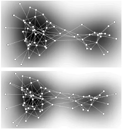
0. The resulting visualizations created by s-SNE with the respective bestgamma-divergence are shown in Fig. 7, where the node layouts by both methods are very similar. In both visualizations we can clearly see two dolphin communities.

In contrast, we demonstrate the failure of selecting γ by minimum cross-validation error (defined with the connected β-divergence in Eq. 23). We have explored the integerγvalues in[₋10,40]. In Fig. 8 (left), we can see that a largerγyields smaller cross-validation error; the smallest error appears at

2_{available at http://www-personal.umich.edu/~mejn/netdata/}

−2 −1 0 1 2 −10000

−9000 −8000 −7000 −6000 −5000

log−likelihood

γ (best γ=0.00) Multinomial

−20 −1 0 1 2 1

2 3 4 5 6x 10

6

negative SM objective

γ (best γ=0.08) Multinomial

−2 −1 0 1 2 −4000

−3500 −3000 −2500 −2000

log−likelihood

γ (best γ=−0.76) PNMF, synthetic data

−20 −1 0 1 2 1000

2000 3000 4000

γ (best γ=−0.80) PNMF, synthetic data

−1 0 1 2 3

−2 0 2 4 6x 10

23

log−likelihood

γ (best γ=1.69) PNMF, swimmer data

1.55 1.6 1.65 1.7 1.75

−10 0 1 2 3 5

10 15x 10

10

γ (best γ=1.63) PNMF, swimmer data

1.55 1.6 1.65 1.7 1.75

−2 −1 0 1 2 4000

6000 8000 10000 12000

log−likelihood

γ (best γ=−0.60)

γ−NE

−2 −1 0 1 2 1000

2000 3000 4000 5000 6000 7000

γ (best γ=−1.04)

γ−NE

Fig. 6. Selecting the bestγ-divergence: (1st row) for multinomial data, (2nd row) in PNMF for synthetic data, (3rd row) in PNMF for theswimmer dataset, and (4th row) in s-SNE for thedolphins dataset; (left column) using MEDAL and (right column) using score matching of EDA. The red star highlights the peak and the small subfigures in each plot shows the zoom-in around the peak. The sub-figures in the 3rd row zoom in the area near the peaks.

γ= 40. However, the resulting s-SNE visualization by using γ= 40in Fig. 8 (right) is much worse than the ones by using our proposed methods (Fig. 7) in terms of identifying the two dolphin communities.

V. CONCLUSIONS

We have presented a new method called MEDAL to au-tomatically select the best information divergence in a para-metric family. Our selection method is built upon a statistical learning approach, where the divergence is learned as the result of standard density parameter estimation. Maximizing the likelihood of the Tweedie distribution is a straightforward

way for selecting β-divergence, which however has some

(10)

Fig. 7. Visualization of thedolphinssocial network with the bestγusing (top) MEDAL and (bottom) score matching of EDA. Dolphins and their social connections are shown by circles and lines, respectively. The background illustrates the node density by the Parzen method [45].

Fig. 8. Selecting the best γ by minimum cross-validation error for the dolphins social network: (left) logorithm of cross-validation errors for variousγvalues, (right) visualization of thedolphinssocial network with

γ= 40.

selection for the parameter over a wider range. The new

method has been extended to α-divergence selection by a

nonlinear transformation. Furthermore, we have provided new results that connect the γ- and β-divergences, which enable us to extend the selection method to non-separable cases. The extension also holds for Rényi divergence with similar relationship to α-divergence. As a result, our method can be applied to most commonly used information divergences in learning.

We have performed extensive experiments to show the accuracy and applicability of the new method. Comparison on synthetic data has illustrated that our method is superior to Maximum Tweedie Likelihood, i.e., it finds the ground truth as accurately as MTL, while being defined on all values of β and being less prone to numerical problems (no abrupt changes in the likelihood). We also showed that a previous estimation approach by Score Matching on Exponential Divergence dis-tribution (ED, i.e., EDA before augmentation) is not accurate, especially for β < 0. In the application to NMF, we have provided experimental results on various kinds of data

includ-ing audio and stock prices. In the non-separable cases, we have demonstrated selecting γ-divergence for synthetic data, Projective NMF, and visualization by s-SNE. In those cases where the correct parameter value is known in advance for the synthetic data, or there is a wide consensus in the application community on the correct parameter value for real-world data, the MEDAL method gives expected results. These results show that the presented method has not only broad applications but also accurate selection performance. In the case of new kinds of data, for which the appropriate information divergence is not known, the MEDAL method provides a disciplined and rigorous way to compute the optimal parameter values.

In this paper we have focused on information divergence for vectorial data. There exist other divergences for higher-order tensors, for example, LogDet divergence and von Newmann divergence (see e.g. [46]) that are defined over eigenvalues of matrices. Selection among these divergences remains an open problem.

Here we mainly consider a positive data matrix and selecting the divergence parameter in(_−∞,+_∞). Tweedie distribution has no support for zero entries when β < 0 and thus gives zero likelihood of the whole matrix/tensor by independence. In future work, extension of EDA to accommodate nonnegative data matrices could be developed forβ ≥0.

MEDAL is a two-phase method: the β selection is based

on the optimization result ofµ. Ideally, both variables should be selected by optimizing the same objective. For maximum likelihood estimator, this requires that the negative log-likelihood equals the β-divergence, which is however

infea-sible for all β due to intractability of integrals. Non-ML

estimators could be used to attack this open problem. The EDA distribution family includes the exact Gaussian, Gamma, and Inverse Gaussian distributions, and approximated Poisson distribution. In the approximation we used the first-order Stirling expansion. One could apply higher-first-order expan-sions to improve the approximation accuracy. This could be implemented by further augmentation with higher-order terms around β_→0.

VI. ACKNOWLEDGMENT

This work was financially supported by the Academy of Fin-land (Finnish Center of Excellence in Computational Inference Research COIN, grant no 251170; Zhirong Yang additionally by decision number 140398).

APPENDIXA

INFINITE SERIES EXPANSION INTWEEDIE DISTRIBUTION

In the series expansion, an EDM random variable is

repre-sented as a sum of Gindependent Gamma random variables

x= PGg yg, where G is Poisson distributed with parameter

λ=_φ(2µ2−₋p_p); and the shape and scale parameters of the Gamma distribution are₋aandb, witha= 2₁₋−_ppandb=φ(p₋1)µp−1_.

The pdf of the Tweedie distribution is obtained analytically at x = 0 as e− µ

2−p

φ(2−p)_{. For} _{x >} ₀ _{the function} _f₍_{x, φ, p}_{) =}

1 x

P∞

j=1Wj(x, φ, p), where for1< p <2

Wj =

x−ja₍_p

−1)ja

(11)

and for p >2

This infinite summation needs approximation in practice. Dunn and Smyth [35] described an approach to select a subset of these infinite terms to accurately approximate f(x, φ, p). In their approach, Stirling’s approximation of the Gamma functions are used to find the index j which gives the highest value of the function. Then, in order to find the most significant region, the indices are progressed in both directions until negligible terms are reached.

APPENDIXB

GAUSS-LAGUERRE QUADRATURES

This method (e.g. [47]) can evaluate definite integrals of the form

wherezi is theith root of then-th order Laguerre polynomial

Ln(z), and the weights are given by

The recursive definition of Ln(z)is given by

Ln+1(z) = 1

n+ 1[(2n+ 1−z)Ln(z)−nLn−1(z)], (29)

with L0(z) = 1 and L1(z) = 1₋z. In our experiments, we used the Matlab implementation by Winckel3 _with_n_{= 5000}_.

APPENDIXC

PROOFS OFTHEOREMS2AND3

Lemma 4: arg minzaf(z) = arg minzalnf(z)for a∈R

andf(z)>0.

The proof of the lemma is simply by the monotonicity of ln. Next we prove Theorem 2. For β _∈ R\{−1,0_}, zeroing

3_{available at http://www.mathworks.se/matlabcentral/fileexchange/}

Dropping the constant, and by Lemma 4, the above is equivalent to minimizing comes minimizing γ-divergence (replacingβ withγ; see Eq. (7)).

We can apply the similar technique to prove Theorem 3. Forα∈R\{0,1}, zeroing ∂Dα(x||cµ)

Putting it back, we obtain

Dα(x_||c∗µ) (32)

the above is equivalent to minimization of (forα >0)

1

becomes minimizing Rényi-divergence (replacing α with ρ;

see Eq. (9)).

The proofs for the special cases are similar, where the main steps are given below

• β =γ→0(or α=ρ→1): zeroing ∂Dβ→0(x||cµ)

Putting it back, we obtain

(12)

of P_iµ˜ilnµ˜_x_ii. Adding the constant lnPjxj to the

latter, the objective becomes identical to Dρ→0(x||µ), i.e., DKL(µ||x).

REFERENCES

[1] R. Kompass, “A generalized divergence measure for nonnegative matrix factorization,”Neural Computation, vol. 19, no. 3, pp. 780–791, 2006. [2] I. S. Dhillon and S. Sra, “Generalized nonnegative matrix approxima-tions with Bregman divergences,” inAdvances in Neural Information Processing Systems, vol. 18, 2006, pp. 283–290.

[3] A. Cichocki, H. Lee, Y.-D. Kim, and S. Choi, “Non-negative matrix factorization withα-divergence,” Pattern Recognition Letters, vol. 29, pp. 1433–1440, 2008.

[4] Z. Yang and E. Oja, “Unified development of multiplicative algorithms for linear and quadratic nonnegative matrix factorization,”IEEE Trans-actions on Neural Networks, vol. 22, no. 12, pp. 1878–1891, 2011. [5] G. Hinton and S. Roweis, “Stochastic neighbor embedding,” inAdvances

in Neural Information Processing Systems, 2002, pp. 833–840. [6] L. van der Maaten and G. Hinton, “Visualizing data using t-SNE,”

Journal of Machine Learning Research, vol. 9, pp. 2579–2605, 2008. [7] D. Blei, A. Y. Ng, and M. I. Jordan, “Latent dirichlet allocation,”Journal

of Machine Learning Research, vol. 3, pp. 993–1022, 2001.

[8] I. Sato and H. Nakagawa, “Rethinking collapsed variational bayes inference for lda,” in International Conference on Machine Learning (ICML), 2012.

[9] T. Minka, “Divergence measures and message passing,” Microsoft Research, Tech. Rep., 2005.

[10] H. Chernoff, “A measure of asymptotic efficiency for tests of a hy-pothesis based on a sum of observations,”The Annals of Mathematical Statistics, vol. 23, pp. 493–507, 1952.

[11] S. Amari, Differential-Geometrical Methods in Statistics. Springer Verlag, 1985.

[12] A. Basu, I. R. Harris, N. Hjort, and M. Jones, “Robust and efficient estimation by minimising a density power divergence,” Biometrika, vol. 85, pp. 549–559, 1998.

[13] H. Fujisawa and S. Eguchi, “Robust paramater estimation with a small bias against heavy contamination,” Journal of Multivariate Analysis, vol. 99, pp. 2053–2081, 2008.

[14] A. Cichocki and S.-i. Amari, “Families of alpha- beta- and gamma-divergences: Flexible and robust measures of similarities,” Entropy, vol. 12, no. 6, pp. 1532–1568, 2010.

[15] A. Cichocki, S. Cruces, and S.-I. Amari, “Generalized alpha-beta diver-gences and their application to robust nonnegative matrix factorization,”

Entropy, vol. 13, pp. 134–170, 2011.

[16] I. Csiszár, “Eine informationstheoretische ungleichung und ihre an-wendung auf den beweis der ergodizitat von markoffschen ketten,”

Publications of the Mathematical Institute of Hungarian Academy of Sciences Series A, vol. 8, pp. 85–108, 1963.

[17] T. Morimoto, “Markov processes and the h-theorem,” Journal of the Physical Society of Japan, vol. 18, no. 3, pp. 328–331, 1963. [18] L. M. Bregman, “The relaxation method of finding the common points

of convex sets and its application to the solution of problems in convex programming,” USSR Computational Mathematics and Mathematical Physics, vol. 7, no. 3, pp. 200–217, 1967.

[19] Z. Yang, H. Zhang, Z. Yuan, and E. Oja, “Kullback-leibler divergence for nonnegative for nonnegative matrix factorization,” inProceedings of 21st International Conference on Artificial Neural Networks, 2011, pp. 14–17.

[20] Z. Yang and E. Oja, “Projective nonnegative matrix factorization with

α-divergence,” in Proceedings of 19th International Conference on Artificial Neural Networks, 2009, pp. 20–29.

[21] C. Févotte, N. Bertin, and J.-L. Durrieu, “Nonnegative matrix factor-ization with the Itakura-Saito divergence. With application to music analysis,”Neural Computation, vol. 21, no. 3, pp. 793–830, 2009. [22] B. Jørgensen, “Exponential dispersion models,” Journal of the Royal

Statistical Society. Series B (Methodological), vol. 49, no. 2, pp. 127– 162, 1987.

[23] A. Cichocki, R. Zdunek, A. H. Phan, and S. Amari,Nonnegative Matrix and Tensor Factorization. John Wiley and Sons, 2009.

[24] Y. K. Yilmaz and A. T. Cemgil, “Alpha/beta divergences and Tweedie models,”CoRR, vol. abs/1209.4280, 2012.

[25] A. Hyvärinen, “Estimation of non-normalized statistical models using score matching,”Journal of Machine Learning Research, vol. 6, pp. 695–709, 2005.

[26] D. D. Lee and H. S. Seung, “Learning the parts of objects by non-negative matrix factorization,”Nature, vol. 401, pp. 788–791, 1999. [27] Z. Yuan and E. Oja, “Projective nonnegative matrix factorization for

image compression and feature extraction,” in Proceedings of 14th Scandinavian Conference on Image Analysis, 2005, pp. 333–342. [28] Z. Yang and E. Oja, “Linear and nonlinear projective nonnegative matrix

factorization,”IEEE Transactions on Neural Networks, vol. 21, no. 5, pp. 734–749, 2010.

[29] Z. Lu, Z. Yang, and E. Oja, “Selectingβ-divergence for nonnegative matrix factorization by score matching,” in Proceedings of the 22nd International Conference on Artificial Neural Networks (ICANN 2012), 2012, pp. 419–426.

[30] S. Eguchi and Y. Kano, “Robustifing maximum likelihood estimation,” Institute of Statistical Mathematics, Tokyo, Tech. Rep., 2001. [31] M. Minami and S. Eguchi, “Robust blind source separation by beta

divergence,”Neural Computation, vol. 14, pp. 1859–1886, 2002. [32] A. Rényi, “On measures of information and entropy,” in Procedings

of 4th Berkeley Symposium on Mathematics, Statistics and Probability, 1960, pp. 547–561.

[33] M. Mollah, S. Eguchi, and M. Minami, “Robust prewhitening for ica by minimizing beta-divergence and its application to fastica,” Neural Processing Letters, vol. 25, pp. 91–110, 2007.

[34] H. Choi, S. Choi, A. Katake, and Y. Choe, “Learning alpha-integration with partially-labeled data,” inProc. of the IEEE International Confer-ence on Acoustics, Speech, and Signal Processing, 2010, pp. 14–19. [35] P. K. Dunn and G. K. Smyth, “Series evaluation of Tweedie exponential

dispersion model densities,”Statistics and Computing, vol. 15, no. 4, pp. 267–280, 2005.

[36] ——, “Tweedie family densities: methods of evaluation,” inProceedings of the 16th International Workshop on Statistical Modelling, 2001. [37] A. Hyvärinen, “Some extensions of score matching,”Comput. Stat. Data

Anal., vol. 51, no. 5, pp. 2499–2512, 2007.

[38] C. Févotte and J. Idier, “Algorithms for nonnegative matrix factorization with the beta-divergence,”Neural Computation, vol. 23, no. 9, 2011. [39] C. F. V. Tan, “Automatic relevance determination in nonnegative matrix

factorization with the β-divergence,” IEEE Transactions on Pattern Analysis and Machine Intelligence, 2013, accepted, to appear. [40] T. Hofmann, “Probabilistic latent semantic indexing,” inInternational

Conference on Research and Development in Information Retrieval (SIGIR), 1999, pp. 50–57.

[41] Z. Yang and E. Oja, “Quadratic nonnegative matrix factorization,”

Pattern Recognition, vol. 45, no. 4, pp. 1500–1510, 2012.

[42] D. Donoho and V. Stodden, “When does non-negative matrix factoriza-tion give a correct decomposifactoriza-tion into parts?” inAdvances in Neural Information Processing Systems 16, 2003, pp. 1141–1148.

[43] V. Y. F. Tan and C. Févotte, “Automatic relevance determination in nonnegative matrix factorization,” in Proceedings of 2009 Workshop on Signal Processing with Adaptive Sparse Structured Representations (SPARS’09), 2009.

[44] Z. Yang, Z. Zhu, and E. Oja, “Automatic rank determination in projective nonnegative matrix factorization,” in Proceedings of the 9th Interna-tional Conference on Latent Variable Analysis and Signal Separation (LVA2010), 2010, pp. 514–521.

[45] E. Parzen, “On Estimation of a Probability Density Function and Mode,”

The Annals of Mathematical Statistics, vol. 33, no. 3, pp. 1065–1076, 1962.

[46] B. Kulis, M. A. Sustik, and I. S. Dhillon, “Low-rank kernel learning with bregman matrix divergences,” Journal of Machine Learning Research, vol. 10, pp. 341–376, 2009.

(13)

Onur Dikmen(M’09) received his B.Sc., M.Sc. and Ph.D. degrees from the Department of Computer Engineering, Bo˘gaziçi University, Turkey.

He worked at Télécom ParisTech, France as a CNRS research associate. He is currently with the Department of Information and Computer Science at Aalto University, Finland. His research interests include statistical signal processing, machine learn-ing, and approximate Bayesian inference. He works on inference and optimization in Markov random fields, Bayesian source modeling and nonnegative matrix factorization with application to audio source separation and sound event detection.

Zhirong Yang(S’05-M’09) received his Bachelor and Master degrees from Sun Yat-Sen University, China in 1999 and 2002, and Doctoral degree from Helsinki University of Technology, Finland in 2008, respectively. Presently he is a Docent and postdoc-toral researcher with the Department of Information and Computer Science at Aalto University. His cur-rent research interests include pattern recognition, machine learning, computer vision, and information retrieval, particularly focus on nonnegative learning, information visualization, optimization, discrimina-tive feature extraction and visual recognition. He is a member of the Institute of Electrical and Electronics Engineers (IEEE) and the International Neural Network Society (INNS).

Erkki Oja (S’75-M’78-SM’90-F’00) received the D.Sc. degree from Helsinki University of Technol-ogy in 1977. He is Director of the Computational In-ference Research Centre and Professor of Computer Science at the Laboratory of Computer and Infor-mation Science, Aalto University, Finland. He holds an honorary doctorate from Uppsala University, Sweden. He has been research associate at Brown University, Providence, RI, and visiting professor at the Tokyo Institute of Technology, Japan. He is the author or coauthor of more than 300 articles and book chapters on pattern recognition, computer vision, and neural computing, and three books: "Subspace Methods of Pattern Recognition" (New York: Research Studies Press and Wiley, 1983), which has been translated into Chinese and Japanese; "Kohonen Maps" (Amsterdam, The Netherlands: Elsevier, 1999), and "Independent Component Analysis" (New York: Wiley, 2001; also translated into Chinese and Japanese). His research interests are in the study of principal component and independent component analysis, self-organization, statistical pattern recognition, and applying machine learning to computer vision and signal processing.