IMPROVED TOPOGRAPHIC MODELS VIA CONCURRENT AIRBORNE LIDAR AND
DENSE IMAGE MATCHING
G. Mandlburgera, b∗, K. Wenzelc, A. Spitzerd, N. Haalab, P. Gliraa, e, N. Pfeifera
a
TU Vienna, Department of Geodesy and Geoinformation, Vienna, Austria -(gottfried.mandlburger, philipp.glira, norbert.pfeifer)@geo.tuwien.ac.at
bUniversity of Stuttgart, Institute for Photogrammetry, Stuttgart, Germany
-(gottfried.mandlburger, norbert.haala)@ifp.uni-stuttgart.de
c
nFrames GmbH, Stuttgart, Germany - [email protected]
d
RIEGLLaser Measurement Systems, Horn, Austria - [email protected]
e
Siemens AG, Corporate Technology (CT), Vienna, Austria, [email protected]
Commission II, WG II/1
KEY WORDS:airborne laser scanning, aerial images, digital surface model, sensor orientation, data fusion
ABSTRACT:
Modern airborne sensors integrate laser scanners and digital cameras for capturing topographic data at high spatial resolution. The capability of penetrating vegetation through small openings in the foliage and the high ranging precision in the cm range have made airborne LiDAR the prime terrain acquisition technique. In the recent years dense image matching evolved rapidly and outperforms laser scanning meanwhile in terms of the achievable spatial resolution of the derived surface models. In our contribution we analyze the inherent properties and review the typical processing chains of both acquisition techniques. In addition, we present potential synergies of jointly processing image and laser data with emphasis on sensor orientation and point cloud fusion for digital surface model derivation. Test data were concurrently acquired with theRIEGLLMS-Q1560 sensor over the city of Melk, Austria, in January 2016 and served as basis for testing innovative processing strategies. We demonstrate that (i) systematic effects in the resulting scanned and matched 3D point clouds can be minimized based on a hybrid orientation procedure, (ii) systematic differences of the individual point clouds are observable at penetrable, vegetated surfaces due to the different measurement principles, and (iii) improved digital surface models can be derived combining the higher density of the matching point cloud and the higher reliability of LiDAR point clouds, especially in the narrow alleys and courtyards of the study site, a medieval city.
1. INTRODUCTION
Airborne LiDAR (Light Detection And Ranging), also referred to as Airborne Laser Scanning (ALS), has become the state-of-the-art data acquisition method for topographic mapping due its capability to provide dense and reliable height information and to penetrate vegetation through small gaps in the foliage. The ac-ceptance of the technique is underlined by a number of facts: (i) national mapping agencies all over the world have started, have already completed, or are updating their country-wide data acqui-sition, (ii) approximately 20k articles have been published since the turn of the century according to ScienceDirect when searched for the keywords ”lidar” and ”topography”, and (iii) several text books on the topic have been published (Shan and Toth, 2008; Vosselman and Maas, 2010).
Recent advances in digital photogrammetry and computer vision have brought passive imagery back into the focus for area-wide terrain elevation mapping. Especially the introduction of sophis-ticated Dense Image Matching (DIM) techniques (Remondino et al., 2014; Haala and Rothermel, 2012; Hirschmuller, 2008) pro-viding elevations for each image pixel has increased the achiev-able point density and led to surface models with a point spacing equal to the ground sampling distance (GSD) of the images (typ-ically 5-20 cm).
Therefore, several advanced 3D mapping sensors feature laser
∗Corresponding author: [email protected]
scanners and (RGB) camera systems on the same airborne plat-form. One obvious advantage of such a hybrid sensor system is that the (monochromatic) laser echoes can be enriched by color information from synchronously acquired images. Beyond that, the combination of active laser and passive image sensors may open new opportunities for improving topographic data w.r.t. completeness, density, geo-referencing quality, precision, relia-bility, (point cloud) classification, object detection, surface recon-struction, and processing speed. For exploiting the full potential of the respective data sources it is necessary to fully understand their properties.
Whereas general comparisons of airborne LiDAR and DIM for terrain modeling and forestry applications were already published (Ressl et al., 2016; Vastaranta et al., 2013), this contribution specifically focuses on the potentials and challenges of simulta-neous data acquisition from the same platform. This rules out that differences in the products are due to changes of the scene (construction activities, phenological state of vegetation, etc.) or changes in environmental factors (atmosphere, sun position, etc.).
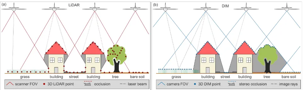
Figure 1. Schematic drawing of data acquisition based on airborne LiDAR (a) and DIM (b)
laser scans (Skaloud and Lichti, 2006; Glira et al., 2015a) and images (Kraus, 2007; F¨orstner and Wrobel, 2016). However, the simultaneous use of data from LiDAR and image matching plies a second level of relative orientation between scans and im-ages which is important to consider when jointly using the point clouds of both acquisition techniques for deriving products (sur-face and terrain models, orthophoto mosaics, etc.). Hence, one of the main goals of this paper is to examine the different properties of the point clouds obtained from LiDAR and image matching as only those areas must be used for mutual orientation of scans and images where no sensor related differences exist. In low vege-tation, for instance, inherent height differences between the two techniques have been reported by Ressl et al. (2016). Building on that, new approaches for jointly processing scans and images are developed.
This article, therefore, briefly reviews the techniques and their properties in Section 2 and presents the typical individual data processing chains as well as proposals for integrated workflows in Section 4. The setup of an experimental data acquisition with a hybrid LiDAR/imaging sensor is described in Section 3 and the respective results are presented and discussed in Section 5. The major findings and recommendations are finally summarized in Section 6.
2. TECHNIQUES AND PROPERTIES
In this section, the principles of mapping topography with LiDAR and DIM are shortly summarized and the properties of the indi-vidual measurement techniques are discussed. This will result in requirements for joint data processing.
2.1 Airborne LiDAR
Airborne LiDAR is an active polar measurement system which uses short laser pulses for time-of-flight range detection. The lin-ear LIDAR technology utilized inRIEGLLiDAR systems makes use of echo digitization and either full waveform analysis or on-line waveform processing (Ullrich and Pfennigbauer, 2016). Sys-tems using this technology provide accurate 3D point clouds as well as additional attributes per point including calibrated ampli-tude and reflectance readings, but also attributes derived from the shape of the echo waveforms itself. One of the specific strengths of LIDAR technology is its multi-target capability enabling the penetration of vegetation to reveal objects below the canopy and to provide data from the ground for deriving a high resolution digital terrain model (cf. Figure1a).
2.2 Dense Image Matching
Driven by advances in digital camera system technology and al-gorithms, limits of automatic image based 3D surface reconstruc-tion were pushed to a very high level regarding precision, ro-bustness, and processing speed (Remondino et al., 2014; Haala and Rothermel, 2012). Starting from a set of images and their corresponding camera parameters (i.e. interior and exterior ori-entation), multi-view stereo (MVS) algorithms first compute so-called disparity maps applying suitable stereo matching algo-rithms (Hirschmuller, 2008; Yan et al., 2016). As a result, stereo correspondences between pixels across image pairs are estab-lished.
A set of images rectified to epipolar geometry, also referred to as stereo vision geometry, constitutes the typical input for dense stereo matching. In this case potential correspondences are lo-cated on identical rows across an image pair. Matching each im-age against multiple proximate imim-ages then generates redundant depth observations, which leads to so-called depth maps. Thus, each single pixel of an image block provides one or more cor-responding 3D coordinates. The resulting dense point cloud can subsequently be filtered during DSM generation. If suitable re-dundancy is available from multiple views, state-of-the-art algo-rithms can reconstruct surface geometry at a resolution and accu-racy which corresponds to the resolution of the available imagery.
2.3 Point cloud properties
The main characteristics of LiDAR and DIM are summarized in Table 1 and exemplary consequences for the acquired 3D point clouds are visualized in Figure 2 and Figure 3. Although the data samples are taken from the specific flight block detailed in Section 3, the aim is to highlight general properties of LiDAR and image matching point clouds.
Airborne LiDAR Dense Image Matching data acquisition multi-sensor system (GNSS+IMU+scanner+camera)
light source active (laser) passive (solar radiation)
measurement principle time-of-flight image ray intersection measurement rays per point 1 (polar system) >2 (multi-view stereo) target detection multiple targets per pulse topmost surface
radiometry mono-spectral (@laser wavelength) multi-spectral (IR-R-G-B)
typical point spacing 20-50 cm 5-20 cm
preconditions (diffuse) object reflectance texture (image contrast)
typical height precision 2-3 cm 0.5-2 x GSD
Table 1. LiDAR/DIM characteristics and properties
color tones in Figure 2b and from the vertical section in Figure 2c and has a concrete implication for mutual orientation of scans and images. Although grass appears smooth in LiDAR and DIM datasets, the sensed surfaces exhibit a systematic bias and, thus, correspondences between images and scans must be avoided for these low vegetation areas.
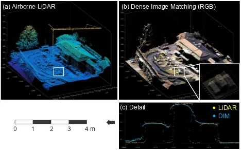
Figure 3a and 3b show that the LiDAR dataset captures more points of the leafless tree and that the construction crane visible in the LiDAR point cloud is missing in the DIM dataset (Fig-ure 3b). The polar meas(Fig-urement principle of LiDAR allows the detection of one or multiple returns along a single laser ray path. Multiple laser returns occur if the laser beam cone hits targets smaller than the laser footprint in different distances along the ray path (e.g. power lines, twigs, branches). As opposed to this, surface reconstruction based on (multi-view) stereo matching re-quires that the same object is seen from at least two camera
po-Colorized DIM point cloud
beach volleyball court
soccer field running track
A B
LiDAR DIM
Height differences: DIM-LiDAR
(b) (a)
(c)
[m]
Figure 2. Penetration depths of LiDAR and DIM over different surfaces, (a) RGB-colored DIM point cloud featuring different surface types (white boxes), (b) color coded height differences
LiDAR minus DIM, (c) vertical section of profile AB
(b) Dense Image Matching (RGB) (a) Airborne LiDAR
DIM
LiDAR
0 1 2 3 4 m
(c) Detail
Figure 3. Comparison of 3D point clouds from LiDAR and DIM, (a) LiDAR, (b) DIM (RGB), (c) vertical section of detail
(white rectangle) showing a pile of construction material
sitions. Whereas modern digital cameras allow high along-track overlaps (typically≥80 %) minimizing the occlusion problem, still polar measurements are advantageous whenever the object appearance changes rapidly when seen from different positions (i.e. semi-transparent objects like vegetation, crane bars), when the objects are in motion (vehicles, pedestrians, etc.), or in very narrow canyons. Figure 3c gives an example for the latter. The detail shows three piles of construction material (height: 1-2 m, width: 1 m) with a narrow 50 cm gap between each pile. Whereas the laser beam occasionally reaches the ground between the piles, both stereo-occlusion and cast shadows prevent the generation of DIM ground points. Whereas this is an extreme example, the same situation also occurs in narrow alleys and small courtyards surrounded by high buildings.
Figure 3c also shows artificial ramps around the piles caused by the smoothness constraint within the DIM framework. The heights between the ground level and the pile’s top level show a smooth transition in the DIM point cloud compared to the more abrupt height jump in the LiDAR point cloud. Within this tran-sition zone, flying points occur in the DIM dataset which do not represent real targets. The simultaneous use of laser scanners and cameras shows a clear potential in this respect, as the higher relia-bility of the LiDAR points can be utilized for DIM-based surface reconstruction, either within image matching or later during point cloud fusion and DSM derivation.
Also the LiDAR point cloud shows averaging effects at the boundary of piles as well caused by the finite laser footprint hit-ting both vertical and horizontal surface parts. The respective laser echo is calculated along the laser beam axis with an aver-aged distance derived from the broadened echo waveform. Anal-ysis of the backscattered waveform allows the identification of such low quality points as the width of the echo is much longer than the width of the emitted pulse in such situations.
Figures 2c and 3b/c show a clear advantage of DIM over LiDAR, namely the higher point density. To sum it up, advantages of Li-DAR w.r.t. higher reliability and less occlusion are compensated by the higher point density of DIM. Together with inherent dif-ferences concerning the penetration of semi-transparent objects, these properties need to be considered during data processing to achieve optimal results.
3. DATA ACQUISITION
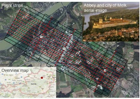
Abbey and city of Melk aerial image
Overview map Flight strips
Figure 4. Study area city of Melk (Austria), center: planned flight trajectories (black lines) and camera positions (red circles), upper right: aerial image of the abbey and city of Melk,
bottom left: location of study area (red circle) within Austria
was chosen because it contains different types of landscape com-prising deciduous and coniferous forests, cropland, water bodies, as well as suburban and urban areas, including the challenging narrow alleys in the historic part of the city of Melk (Figure 4).
In January 2016 (leave-off season), sample data of 9 parallel flight lines were acquired from 600 m above ground level (AGL) with theRIEGLLMS-Q1560 compact, dual channel full wave-form laser scanner system mounted on a Diamond DA42 light aircraft. Three additional cross strips were captured to enable op-timum flight block adjustment. The system features a fully inte-grated aerial medium format camera and a high-grade INS/GNSS system.
The two laser channels of the LMS-Q1560 have a field of view (FOV) of 58◦ and are rotated around the vertical axis of the system providing a ±8◦ forward/backward looking capability at the border of the scan strips. The sample data were ac-quired with a laser pulse repetition rate of 2 x 400 kHz at a flying speed of 110 knots. This resulted in an average point density of 14 points/m2.
The aerial images were captured with a PhaseOne iXU-R 180, a 80 MPix RGB CCD camera equipped with forward motion com-pensation. Image acquisition was carried out with a 50 mm lens providing a FOV of 56.2◦and a nominal image and side overlap of 80%. At 600 m AGL the resulting GSD is 6.2 cm.
4. DATA PROCESSING
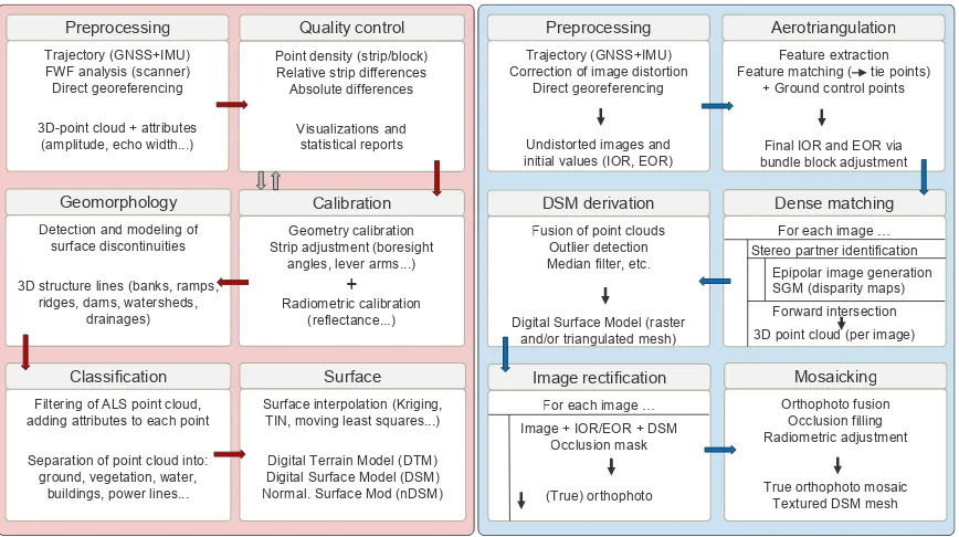
Typical processing chains for LiDAR and DIM are summarized in Figure 5 and briefly discussed in Sections 4.1 and 4.2. Integrated data processing options are presented in Section 4.3.
4.1 LiDAR workflow
During data acquisition, the measurements of the inertial navi-gation system and the laser scanner are time-stamped based on a common time frame. In post-processing the IMU and GNSS measurements are combined to a trajectory providing the posi-tion and attitude of the platform over time.
The (line) angle of each laser shot is determined during data ac-quisition. For full-waveform scanners, the range of each laser
echo is calculated offline in post-processing. First, the precise time stamp of each echo is calculated within the full waveform analysis (Ullrich and Pfennigbauer, 2011). For flight missions with ranges exceeding the maximum unambiguous measurement range, more than one laser pulse is in the air at a time. This is re-ferred to as multiple-time-around (MTA). The correct association of each received echo signal to its causative emitted laser pulse is established during the MTA resolution (Rieger, 2014).
Based on the trajectory, the system’s mounting calibration (i.e. position/orientation offset between trajectory and scanner co-ordinate system), and the range and angle measurements of the laser scanner, the 3D coordinates of each detected laser echo can be calculated. Any error in the trajectory solution, the mounting calibration, or the sensor calibration will cause an offset between point clouds of different flight strips in overlapping areas. Re-spective discrepancies are detected within standard quality con-trol procedures (Ressl et al., 2008). If the deviations exceed ac-ceptable limits, a typical LiDAR workflow also includes an ad-justment to minimize the offsets between the strips (Glira et al., 2015a).
The remaining part of the LiDAR processing pipeline consists of ground-point filtering, break line detection, and surface and terrain model interpolation (Pfeifer and Mandlburger, 2008). For the study at hand, the described workflow was accomplished with the RIEGLRiPROCESS software suite and the scientific laser scanning software OPALS (Pfeifer et al., 2014).
4.2 DIM workflow
For the Dense Image Matching the SURE workflow (Rother-mel et al., 2012; Wenzel et al., 2013) was utilized, which is based on a dense stereo matching algorithm in a multi-view stereo environment (Figure 5). After image orientation via bun-dle block adjustment, pixel-wise disparity information is deter-mined for every stereo pair using a variation of the Semi Global Matching (SGM) algorithm (Hirschmuller, 2008) which enables dense stereo through an efficient approximated global optimiza-tion while aiming to preserve sharp edges and discontinuities.
Opposed to the original SGM method, a hierarchical strategy is used within the SURE workflow (the tSGM approach) where the disparity search range is reduced successively to reduce complex-ity. This is particularly beneficial for scenes with large parallax variations. Thereafter, the dense disparity information of each stereo pair is utilized within a multi-stereo forward intersection where for every pixel all available correspondences are used to generate a 3D point. The dense disparity maps enable correspon-dence linking through the epipolar geometry as well as outlier rejection and noise reduction. Consequently, one 3D point is gen-erated for every pixel featuring sufficient stereo information.
Trajectory (GNSS+IMU) Feature matching ( tie points)
+ Ground control points
Final IOR and EOR via bundle block adjustment 3D point cloud (per image) Fusion of point clouds
Outlier detection Median filter, etc.
Digital Surface Model (raster and/or triangulated mesh)
3D-point cloud + attributes (amplitude, echo width...) Detection and modeling of
surface discontinuities
3D structure lines (banks, ramps, ridges, dams, watersheds,
drainages)
Filtering of ALS point cloud, adding attributes to each point
Separation of point cloud into: ground, vegetation, water,
Figure 5. Schematic diagram of typical LiDAR and DIM processing chains
The resulting product is a 2.5D DSM represented either by a height image raster or a point cloud containing the averaged color information of the original imagery with up to 4 bands. Due to the properties of the tSGM approach, sharp edges can be pre-served while being able to provide depth information in radiomet-rically challenging areas - such as in the presence of image noise. The height precision depends on both the geometric configura-tion (image scale/GSD, intersecconfigura-tion angle, redundancy) and the radiometric information (texture quality). As a property of this passive approach, a sufficient signal-to-noise ratio is required to provide reliable surface information.
The DSM is generated in tiles, followed by an optional inter-polation across multiple tiles. The SURE workflow furthermore provides capabilities for the production of True Orthophotos and triangulated surfaces (meshes) which are based on the extracted geometry. For the True Orthophotos, the locally involved images are rectified and merged according to the DSM. Meshes can ei-ther be derived in 3D space or from the DSM, as used within this study for visualization purposes. For DSM generation and the production of True Orthophoto or meshes, also additional or modified data can be incorporated into the processing pipeline. Within this study, the LiDAR point clouds were introduced as described in Section 4.3.2.
4.3 Hybrid data processing
4.3.1 Integrated sensor orientation Strip adjustment (SA) of LiDAR strips and bundle block adjustment (BBA) of aerial images are usually performed independently. As a consequence, systematic discrepancies between the DIM and LiDAR point clouds can be observed in general. To minimize these discrep-ancies, LiDAR data and image data have to be oriented and cal-ibrated in a single hybrid adjustment, in which SA and BBA are integrated in a rigorous way.
The strip adjustment of LiDAR strips, which serves as a founda-tion for the hybrid adjustment proposed herein, was previously published in Glira et al. (2015a), Glira et al. (2015b), and Glira et al. (2016). Summarizing, this strip adjustment method . . .
• establishes correspondences within the overlapping parts of the LiDAR strips in an iterative manner as in the well-known Iterative Closest Point (ICP) algorithm
• takes the original scanner and trajectory measurements as mandatory input data
• takes ground-truth data, e.g. ground control points, as op-tional input
• performs an on-the-job calibration of the entire LiDAR multi-sensor system
• corrects the flight trajectory errors individually for each strip As can be seen in Figure 6, for the strip adjustment correspon-dences are established between (a) overlapping LiDAR strips to-LAS) and (b) LiDAR strips and ground-truth data (LAS-to-GTD). The cost function minimizes the sum of squared (point-to-plane) distances between all these correspondences simulta-neously. The unknowns are the mounting calibration, the flight trajectory errors, and calibration parameters of the laser scanner.
Building on the above SA framework, BBA of aerial images was integrated in a hybrid adjustment. For this, additional cor-respondences are established between (c) the tie points of
over-strip 2
lapping images (IMG-to-IMG), (d) image tie points and ground-truth data, e.g. GCPs (IMG-to-GTD), and (e) image tie points and LiDAR strips (IMG-to-LAS). Whilst the correspondence cat-egories (a) and (b) are commonly used in SA, and (c) and (d) are commonly used in BBA, the correspondences of category (e) are the important connecting link between the LiDAR strips and the aerial images. By minimizing the squared point-to-plane dis-tances (point from images, plane from LiDAR strips) for each of these correspondences, the relative orientation between the LiDAR strips and the aerial images is optimized in the hybrid adjustment. Additional unknowns in the hybrid adjustment are, thus, the exterior and inner orientations of the photos and the co-ordinates of the image tie points.
4.3.2 Point cloud fusion The fusion of point clouds from Li-DAR and DIM follows the general strategy as described in sec-tion 4.2. The point clouds of both sources are utilized simul-taneously in a 2.5D grid filtering step where the highest points are clustered and filtered using a median based approach. For the DIM point cloud, a DSM point cloud (DIM-DSM) in the identical raster scheme and GSD is used while preserving only the points with highest quality by setting the minimum number of consis-tent observations per cell to 8. Wherever the DIM results do not meet this rigorous criterion, remaining gaps are complemented by LiDAR points. Besides this constraint, a filter for gross errors (disparity outliers defined by certain area and distance to the sur-face) is used during the extraction of the DSM from the raw DIM point cloud. The resulting DIM-DSM and LiDAR point clouds are then used in a repeated mutual raster filtering step with the minimum observations per cell set to 1. Further filters, such as the speckle filter, are deactivated in order to maintain all points introduced to the fusion process.
Subsequently, the interpolation across multiple tiles is carried out using the path based interpolation proposed by Hirschmuller (2008) which propagates height information from the local height level. This heuristic approach prevents the mixing of roof and ground information for data gaps on the ground, since points are only interpolated from other ground points. This is particularly useful for urban environments where typically roof information is available, while ground surfaces suffer from occlusions and low radiometric information due to shadows.
Even though a focus of this study is the geometric benefit of the fused point cloud, further products benefiting from the improved geometry such as a True Orthophoto and a textured DSM Mesh are produced for comparison. In summary, the following steps are carried out for the generation and fusion of point clouds. Whereas step 1 is carried out with the OPALS software (Pfeifer et al., 2014), all subsequent steps are based on the SURE workflow (Wenzel et al., 2013):
1. Integrated aerial triangulation and LiDAR strip adjustment 2. DIM point cloud generation (raw 3D points)
3. DIM Digital Surface Model extraction (DIM-DSM, inter-mediate product)
4. Final Digital Surface Model extraction (DIM-DSM + Li-DAR)
5. DIM-LiDAR True Orthophoto and DSM mesh extraction
5. RESULTS AND DISCUSSIONS
The processing strategies outlined in Section 4.3 were applied to the city of Melk flight block and the respective results are pre-sented and discussed in the following section.
Initially, the orientation of LiDAR strips and images was carried out independently. The LiDAR flight block was processed with the OPALS software (Pfeifer et al., 2014) based on the approach of Glira et al. (2015a) and image aerial triangulation was per-formed with Trimble Match-AT. For the LiDAR block, the pre-cision was estimated by analyzing the height differences of all overlapping strip pairs within smooth areas. The deviations ex-hibited a robust standard deviationσMAD=1.2 cm. The image
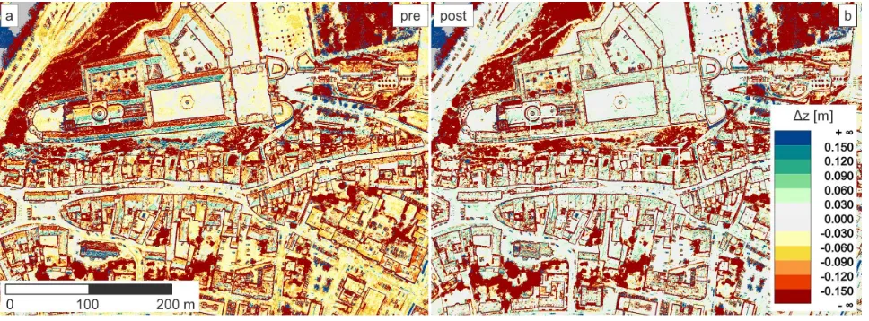
ori-entation was checked at 9800 image tie points and showed a stan-dard deviation of 0.1 pixel (GSD: 6 cm). In contrast to this very good precision of the individual data sources, comparison of the LiDAR-DSM and the DIM-DSM showed unexpected systematic deviations at impervious surfaces (Figure 7a) with a bias (me-dian) of -4.3 cm and a dispersionσ
MAD=4.1 cm. Whereas this represents the situation after orientation of scans and images sep-arately, a substantial improvement could be achieved with the in-tegrated orientation approach described in Section 4.3.1. As can be seen from the dominant whitish colors in Figure 7b the relative discrepancies between the LiDAR and the DIM point cloud could effectively be reduced (bias: 0.2 cm, dispersion:σ
MAD=3.3 cm).
The resulting image orientations were subsequently used as start-ing point for the DIM point cloud generation and the point cloud fusion approach described in Section 4.3.2. Figure 7b still re-veals areas with pronounced vertical deviations between the Li-DAR and the DIM dataset of more than 10 cm. Most of the large discrepancies occur in vegetated areas and rather stem from the different measurement principle than from sensor or data process-ing related deficiencies. Apart from this, problematic areas (white boxes marked in Figure 7b) were detected and are discussed be-low.
The harsh lighting conditions during data acquisition (very bright and low standing winter sun) resulted in cast shadows and caused sub-optimal conditions for DIM surface reconstruction especially in the area of narrow alleys and small inner courtyards. An ex-treme example is displayed in Figure 8. The colorized DIM point cloud of two building blocks, each with a small inner courtyard, is displayed in Figure 8a. At the transition from roof-level to courtyard-level a large tree (only visible in the sectional view of Figure 8b) causes void areas in the DIM point cloud. Further-more, despite the high image and strip overlap of 80 %, the low image contrast prohibits proper DIM reconstruction of the bal-cony located at the first floor level of the inner, eastern wall of the eastern building block while the active, polar LiDAR technique allows proper reconstruction (cf. Figure 8b). Finally, the DIM point cloud shows smoothing effects at the roof ridges. Although, in general, LiDAR is also prone to smoothing, the effect is limited to the laser footprint as already discussed in Section 2.3.
Figure 7. Color coded height differences LiDAR vs. DIM before (a) and after (b) simultaneous orientation of scans and images
meshes.
(a)
a
(b)
Figure 8. Comparison of a complex profile, (a) plan view of RGB colored DIM point cloud, (b) section view, LiDAR points
(red), DIM points (blue)
Figure 9. Ambient occlusion shading of hybrid LiDAR-DIM DSM mesh; detail: narrow alley within the abbey with roof points stemming from DIM and ground floor points from LiDAR
6. CONCLUSIONS
An experiment based on the simultaneous acquisition of airborne LiDAR and photos was conducted. Point clouds acquired from either source, i.e. direct georeferencing of the polar LiDAR
mea-surements and multiple ray forward intersection after dense im-age matching, were compared. Given the higher sampling of the image in comparison to the LiDAR, also the point cloud from dense image matching has a higher density (DIM: 280 points/m2 vs. LiDAR: 14 points/m2). Although the image matching point cloud is denser by a factor of 20, the roof ridges appear rounded off more in the DIM point cloud than in the LiDAR point cloud (Figure 8). The simultaneous acquisition allowed investigating differences of the sensing technologies, rather than comparing two epochs of a changing world, acquired with two different methods.
The simultaneous acquisition of airborne LiDAR and photos and subsequent computation of point clouds from either source in-dependently confirmed expected differences for tall vegetation (Figure 3a, b). In leaf-off data acquisition, as was the case in the experiment conducted, the crown is captured well by laser scanning. Image matching provided a comparatively incomplete representation. In contrast, under leaf-on conditions, as shown, e.g., by Ressl et al. (2016), both methods capture the top surface of the crown well, but laser scanning also captures the ground surface due to its multi-target capability.
The simultaneous acquisition allowed also to study subtle differ-ences in vegetation. The grass of a soccer field lead to height differences between airborne LiDAR and image matching, with the image matching result lying 4 cm higher. It is noteworthy, that either surface model appeared equally smooth.
Linear structures above the ground are captured by LiDAR, be-cause of the polar measurement principle (e.g. the crane in 3a). Due to the multi-target capability, also the ground below a beam or a wire (along the measurement line of sight) is captured. The DIM used in our experiment, in contrast, assumes that the surface is a function parameterized over (e.g.) image space. Thus, only one height can be reconstructed along the measurement ray.
wavelengths, may provide further examples for mutual comple-tion of the measurement technologies, but were not encountered in this experiment.
The simultaneous acquisition may also have disadvantages. The environmental circumstances (low standing sun and very high contrast) caused suboptimal conditions for image matching, but did – in this case – not influence laser scanning. Flying height above ground, flying date (time and season), strip overlap and im-age overlap, etc., influence the quality of the final products. Op-timal conditions for simultaneous acquisition of airborne LiDAR and photos from one platform may provide additional insight in the advantages of either method. A repeat data acquisition of the study area with the same sensor system but under leaf-on condi-tions is currently being prepared. However, also different typical (i.e. not optimal) acquisition scenarios are required, to better un-derstand the relative contribution of either source.
The different properties of the point clouds from laser scanning and image matching are rooted in the different acquisition tech-nologies and need to be considered in a joint orientation of both data sets. Only hard surfaces are suitable tie elements in a com-bined orientation.
Our investigation also demonstrated the advantage such a simul-taneous acquisition can offer for classification. At hard surfaces, height differences between the two point clouds disappear, thus offering a possibility to support classification of surface materi-als.
ACKNOWLEDGEMENTS
This manuscript was funded by the German Research Founda-tion (DFG) project ’Bathymetrievermessung durch Fusion von Flugzeuglaserscanning und multispektralen Luftbildern’.
References
F¨orstner, W. and Wrobel, B. P., 2016. Photogrammetric Com-puter Vision: Statistics, Geometry, Orientation and Recon-struction. Springer International Publishing, Cham, Switzer-land, pp. 643–725.
Glira, P., Pfeifer, N. and Mandlburger, G., 2016. Rigorous strip adjustment of UAV-based laserscanning data including time-dependent correction of trajectory errors. Photogrammetric Engineering & Remote Sensing82(12), pp. 945–954. Glira, P., Pfeifer, N., Briese, C. and Ressl, C., 2015a. A
Cor-respondence Framework for ALS Strip Adjustments based on Variants of the ICP Algorithm. PFG Photogrammetrie, Fern-erkundung, Geoinformation2015(4), pp. 275–289.
Glira, P., Pfeifer, N., Briese, C. and Ressl, C., 2015b. Rigorous strip adjustment of airborne laserscanning data based on the ICP algorithm. In:ISPRS Annals of the Photogrammetry, Re-mote Sensing and Spatial Information Sciences, Vol. II-3/W5, pp. 73–80.
Haala, N. and Rothermel, M., 2012. Dense Multi-Stereo Matching for High Quality Digital Elevation Models. PFG Photogrammetrie, Fernerkundung, Geoinformation 2012(4), pp. 331–343.
Hirschmuller, H., 2008. Stereo Processing by Semiglobal Match-ing and Mutual Information.IEEE Trans. Pattern Anal. Mach. Intell.30(2), pp. 328–341.
Kraus, K., 2007. Photogrammetry – Geometry from Images and Laser Scans. 2 edn, De Gruyter, Berlin, Germany.
Pfeifer, N. and Mandlburger, G., 2008. Filtering and DTM gener-ation. In: J. Shan and C. Toth (eds),Topographic Laser Rang-ing and ScannRang-ing: Principles and ProcessRang-ing, CRC Press, pp. 307–333.
Pfeifer, N., Mandlburger, G., Otepka, J. and Karel, W., 2014. OPALS – a framework for airborne laser scanning data analy-sis. Computers, Environment and Urban Systems45, pp. 125 – 136.
Remondino, F., Spera, M. G., Nocerino, E., Menna, F. and Nex, F., 2014. State of the art in high density image matching. The Photogrammetric Record29(146), pp. 144–166.
Ressl, C., Brockmann, H., Mandlburger, G. and Pfeifer, N., 2016. Dense Image Matching vs. Airborne Laser Scanning - Com-parison of two methods for deriving terrain models. PFG Photogrammetrie, Fernerkundung, Geoinformation 2016(2), pp. 57–73.
Ressl, C., Kager, H. and Mandlburger, G., 2008. Quality check-ing of ALS projects uscheck-ing statistics of strip differences. In: International Archives of the Photogrammetry, Remote Sens-ing and Spatial Information Sciences, Vol. XXXVII. Part B3b, pp. 253–260.
Rieger, P., 2014. Range ambiguity resolution technique apply-ing pulse-position modulation in time-of-flight scannapply-ing li-dar applications. Optical Engineering53(6), pp. 061614–1 – 061614–12.
Rothermel, M., Wenzel, K., Fritsch, D. and Haala, N., 2012. SURE: Photogrammetric surface reconstruction from imagery. In:Proceedings of the Low Cost 3D Workshop, Berlin. Shan, J. and Toth, C. K. (eds), 2008.Topographic Laser Ranging
and Scanning: Principles and Processing. CRC Press, Boca Raton, FL.
Skaloud, J. and Lichti, D., 2006. Rigorous approach to boresight self-calibration in airborne laser scanning. ISPRS Journal of Photogrammetry and Remote Sensing61(1), pp. 47–59. Ullrich, A. and Pfennigbauer, M., 2011. Echo digitization
and waveform analysis in airborne and terrestrial laser scan-ning. In: D. Fritsch (ed.),Photogrammetric Week ’11, Wich-mann/VDE Verlag, Berlin & Offenbach, pp. 217–228.
Ullrich, A. and Pfennigbauer, M., 2016. Linear LIDAR versus Geiger-mode LIDAR: impact on data properties and data qual-ity. In:Proc. SPIE, Vol. 9832, pp. 983204–1 – 983204–17. Vastaranta, M., Wulder, M. A., White, J. C., Pekkarinen, A.,
Tuominen, S., Ginzler, C., Kankare, V., Holopainen, M., Hyypp¨a, J. and Hyypp¨a, H., 2013. Airborne laser scanning and digital stereo imagery measures of forest structure: Compara-tive results and implications to forest mapping and inventory update. Canadian Journal of Remote Sensing39(5), pp. 382– 395.
Vosselman, G. and Maas, H. (eds), 2010. Airborne and Terres-trial Laser Scanning. Whittles Publishing, UK.
Wenzel, K., Rothermel, M., Haala, N. and Fritsch, D., 2013. SURE – the ifp Software for Dense Image Matching. In: D. Fritsch (ed.),Photogrammetric Week ’13, Wichmann/VDE Verlag, Berlin & Offenbach, pp. 59–70.