Microsoft Press
A Division of Microsoft Corporation One Microsoft Way
Redmond, Washington 98052-6399 Copyright © 2006 by Hitachi Consulting
All rights reserved. No part of the contents of this book may be reproduced or transmitted in any form or by any means without the written permission of the publisher.
Library of Congress Control Number 2006921726
Printed and bound in the United States of America.
1 2 3 4 5 6 7 8 9 QWT 1 0 9 8 7 6
Distributed in Canada by H.B. Fenn and Company Ltd.
A CIP catalogue record for this book is available from the British Library.
Microsoft Press books are available through booksellers and distributors worldwide. For further information about international editions, contact your local Microsoft Corporation office or contact Microsoft Press Inter-national directly at fax (425) 936-7329. Visit our Web site at www.microsoft.com/mspress. Send comments to [email protected].
Microsoft, Excel, Microsoft Press, MSDN, PivotTable, Visual Basic, Windows, Windows NT, and Windows Server are either registered trademarks or trademarks of Microsoft Corporation in the United States and/or other countries. Other product and company names mentioned herein may be the trademarks of their respec-tive owners.
The example companies, organizations, products, domain names, e-mail addresses, logos, people, places, and events depicted herein are fictitious. No association with any real company, organization, product, domain name, e-mail address, logo, person, place, or event is intended or should be inferred.
iii
Part I
Getting Started with Analysis Services
1
Understanding Business Intelligence and Data Warehousing . . . .3
Introducing Business Intelligence . . . 3
What do you think of this book?
We want to hear from you!
Monitoring Cube Activity . . . 326
Profiling Analysis Services Queries . . . 326
Using the Performance Monitor . . . 330
Chapter 12 Quick Reference . . . 333
13
Managing Deployment . . . 335
Reviewing Deployment Options . . . 335
Building a Database . . . 336
Deploying a Database. . . 341
Processing a Database . . . 348
Managing Database Objects Programmatically . . . 351
Working with XMLA Scripts . . . 352
Automating Database Processing . . . 356
Creating a SQL Server Integration Services Package . . . 357
Using the Analysis Services Processing Task . . . 358
Handling Task Failures. . . 359
Scheduling a SQL Server Integration Services Package . . . 361
Planning for Disaster and Recovery . . . 364
Backing Up an Analysis Services Database . . . 365
Restoring an Analysis Services Database . . . 366
Chapter 13 Quick Reference . . . 368
Glossary . . . 369
Index. . . 373
What do you think of this book?
We want to hear from you!
ix
Introduction
Microsoft SQL Server 2005 Analysis Services is the multidimensional online analytical pro-cessing (OLAP) component of Microsoft SQL Server 2005 that integrates relational and OLAP data for business intelligence (BI) analytical solutions. The goal of this book is to show you how to use the tools and features of Analysis Services so you can easily create, manage, and share OLAP cubes within your organization. Step-by-step exercises are included to pre-pare you for producing your own BI solutions.
To help you learn the many features of Analysis Services, this book is organized into four parts. Part I, “Getting Started with Analysis Services,” introduces BI and data warehousing, defines OLAP and the benefits an OLAP tool can bring to a data warehouse, and guides you through the development of your first OLAP cube. Part II, “Design Fundamentals,” teaches you how to design dimensions, measure groups, and measures, and then how to combine and enhance these objects to create an analytical solution that addresses a variety of analytical requirements. Part III, “Advanced Design,” shows you how to use multidimensional expres-sions (MDX) and key performance indicators (KPIs) to further enhance your analytical solu-tions and to query an Analysis Services database. In addition, this part covers special Analysis Services features for advanced dimension design, globalization of analytical solutions, and a variety of interactive features that extend the analytical capabilities of cubes. Part IV, “Produc-tion Management,” explains how to use security to control access to cubes as well as to restrict the data that a particular user can see, how to design partitions to manage database scalability, and how to manage and monitor production databases.
Finding Your Best Starting Point
This book covers the full life cycle of an analytical solution from development to deployment. If you’re responsible only for certain activities, you can choose to read the chapters that apply to your situation and skip the remaining chapters. To find the best place to start, use the fol-lowing table:
If you are Follow these steps
An information consumer who uses OLAP to make decisions
1. Install the sample files as described in “In-stalling and Using the Sample Files.” 2. Work through Parts I and II to become
fa-miliar with the basic capabilities of Analysis Services.
About the Companion CD-ROM
The CD that accompanies this book contains the sample files that you need to complete the step-by-step exercises throughout the book. For example, in Chapter 3, “Building Your First Cube,” you open a sample solution to learn how files are organized in an analytical solution. In other chapters, you add sample files to the solution you’re building so you can focus on a particular concept without spending time to set up the prerequisites for an exercise.
A BI analyst who develops OLAP models and prototypes for business analysis
1. Install the sample files as described in “In-stalling and Using the Sample Files.” 2. Work through Part I to get an overview of
Analysis Services.
3. Complete Part II to develop the necessary skills to create a prototype cube.
4. Review the chapters that interest you in Parts III and IV to learn about advanced fea-tures of Analysis Services and to understand how cubes are accessed by users and how cubes are managed after they are put into production.
An administrator who maintains server re-sources or production migration processes
1. Install the sample files as described in “In-stalling and Using the Sample Files.” 2. Skim Parts I–III to understand the
function-ality that is included in Analysis Services. 3. Complete Part IV to learn how to manage
and secure cube access and content on the server as well as how to configure, monitor, and manage server components and performance.
A BI architect who designs and develops analyt-ical solutions
1. Install the sample files as described in “In-stalling and Using the Sample Files.” 2. Complete Part I to become familiar with the
benefits of Analysis Services.
3. Work through Parts II and III to learn how to create dimensions and cubes and how to implement advanced design techniques. 4. Complete Part IV to understand how to
de-sign cubes that implement the security, per-formance, and processing features of Analysis Services.
System Requirements
To install Microsoft Analysis Services 2005 and to use the samples provided on the compan-ion CD, your computer will need to be configured as follows:
■ Microsoft Windows 2000 Advanced Server, Windows XP Professional, or Windows
Server 2003 with the latest service pack applied.
■ Microsoft SQL Server 2005 Developer or Enterprise Edition with any available service
packs applied. Refer to the Operating System Requirements listed at http://
msdn2.microsoft.com/en-us/library/ms143506(en-US,SQL.90).aspx to determine which edition is compatible with your operating system.
The step-by-step exercises in this book and the accompanying practice files were tested using Windows XP Professional and Microsoft SQL Server 2005 Analysis Services Developer Edition. If you’re using another version of the operating system or a different edition of either applica-tion, you might notice some slight differences.
Installing and Using the Sample Files
The sample files require approximately 52 MB of disk space on your computer. To install and prepare the sample files for use with the exercises in this book, follow these steps:
1. Remove the CD-ROM from its package at the back of this book, and insert it into your CD-ROM drive.
Note If the presence of the CD-ROM is automatically detected and a start window is displayed, you can skip to Step 4.
2. Click the Start button, click Run, and then type D:\startcd in the Open box, replacing the drive letter with the correct letter for your CD-ROM drive, if necessary.
3. Click Install Sample Files to launch the Setup program, and then follow the directions on the screen.
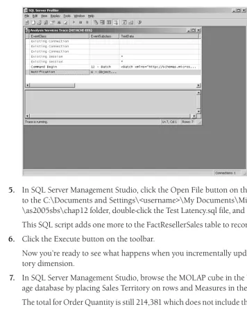
Tip In the C:\Documents and Settings\<username>\My Documents\Microsoft Press\as2005sbs\Answers folder, you’ll find a separate folder for each chapter in which you make changes to the sample files. The files in these folders are copies of these sam-ple files when you comsam-plete a chapter. You can refer to these files if you want to preview the results of completing all exercises in a chapter.
4. Remove the CD-ROM from the drive when installation is complete.
Now that you’ve completed installation of the sample files, you need to follow some additional steps to prepare your computer to use these files.
5. Click the Start button, click Run, and then type C:\Documents and Settings \<username>\My Documents\MicrosoftPress\as2005sbs\Setup\Restore \Restore_databases.cmd in the Open box.
This step attaches the Microsoft SQL Server 2005 database that is the data source for the analytical solution that you will create and use throughout this book.
Now you’re set to begin working through the exercises.
Conventions and Features in This Book
To use your time effectively, be sure that you understand the stylistic conventions that are used throughout this book. The following list explains these conventions:
■ Hands-on exercises for you to follow are presented as lists of numbered steps (1, 2, and
so on).
■ Text that you are to type appears in boldface type.
■ Properties that you need to set in SQL Server Business Intelligence Development Studio
(BIDS) (a set of templates provided in Microsoft Visual Studio) are sometimes displayed in a table as you work through steps.
■ Pressing two keys at the same time is indicated by a plus sign between the two key names,
such as Alt+Tab, when you need to hold down the Alt key while pressing the Tab key.
■ A note that is labeled as Note is used to give you more information about a specific topic.
■ A note that is labeled as Important is used to point out information that can help you
avoid a problem.
■ A note that is labeled as Tip is used to convey advice that you might find useful when
Part I
Getting Started with Analysis
Services
In this part:
Chapter 1: Understanding Business Intelligence and
3
Understanding Business
Intelligence and Data
Warehousing
After completing this chapter, you will be able to:
■ Understand the purpose of business intelligence and data warehousing. ■ Distinguish between a data warehouse and a transaction database. ■ Understand dimensional database design principles.
Microsoft SQL Server 2005 Analysis Services is a tool to help you implement business intelli-gence (BI) in your organization. BI makes use of a data warehouse, often taking advantage of online analytical processing (OLAP) tools. How exactly do BI, data warehousing, OLAP, and Analysis Services relate to each other? In this chapter, you’ll learn the purpose of BI in general, and also some basic concepts of data warehousing in a relational database. In the next chap-ter, you’ll learn how OLAP enhances the capabilities of BI, and how Analysis Services makes both OLAP and relational data available for your BI needs.
Introducing Business Intelligence
BI is a relatively new term, but it is certainly not a new concept. The concept is simply to make use of information already available in your company to help decision makers make decisions better and faster. Over the past few decades, the same goal has gone by many names. In the early 1980s, executive information system (EIS) applications were very popular.
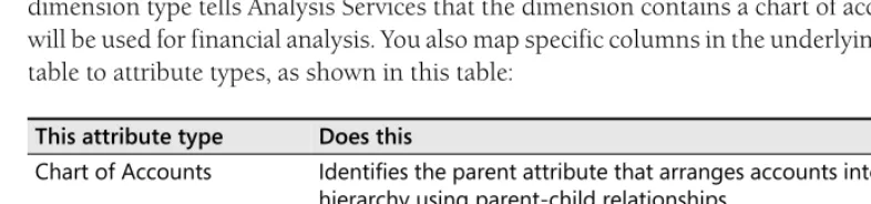
Analysis Services Business Intelligence
Data Warehouse (relational)
OLAP (multidimensional)
Reporting Services
Reporting Services
An EIS, however, often consisted of one person copying key data values from various reports onto a “dashboard” so that an executive could see them at a glance. But the goal was still to help the decision maker make decisions. Later, EIS applications were replaced by decision support system (DSS) applications, which really did essentially the same thing. So what is so different about BI?
The biggest change in the past few decades has been the need to create management reports for all levels of an organization, and all types of decision makers. When you need to provide fast-response reports for many purposes throughout a large organization, having one person type values for another to read is not practical.
One useful way to think about BI is to consider the types of reports—and their respective audi-ences. Typical reports fall into one of the three following general classes.
■ Dashboard reports These are highly summarized, often graphical representations of
the state of the business. The values on a dashboard report are often key performance indicators (KPIs) for an organization. A dashboard report may display a simple summa-tion of month-to-date sales, or it may include complex calculasumma-tions such as profitability growth from the same period of the previous year for the current department compared to the company as a whole. A dashboard often includes comparisons to targets. A dash-board report is often customized for the person viewing the report, showing, for exam-ple, each manager the results for his or her department. Dashboard reports are often used by executives and strategic decision makers.
■ Production reports These are typically large, detailed reports that have the same basic
structure each time they are produced. They may be printed, or distributed online, either in Web-based reports or as formatted files. One advantage of a production report is that the same information can be found in the same place in each report. A production report may consist of one large report showing information about all parts of the com-pany, or it may be “burst” into individual sections delivered to the relevant audience. Production reports are often used by administrators and tactical decision makers.
■ Analytical reports These are dynamic, interactive reports that allow the user to “slice
and dice” the information in any of thousands of ways. As with dashboard reports, ana-lytical reports can display simple summations or complex calculations. They typically allow drill-down to very detailed information, or drill-up to high-level summaries. This type of report is typically used by analysts or “hands-on” managers who want to under-stand all aspects of the situation.
Reviewing Data Warehousing Concepts
A data warehouse is often a core component of a BI infrastructure within an organization. The procedures that you’ll complete throughout this book use a sample data warehouse as the underlying database for the analytical solutions that you’ll build. In this section, you’ll review the characteristics of a data warehouse, the table structures in a data warehouse, and design considerations, but details for building a data warehouse are beyond the scope of this book. For more information about data warehousing, refer to http://msdn.microsoft.com/library /default.asp?url=/library/en-us/createdw/createdw_3r51.asp.
The Purpose of a Data Warehouse
A data warehouse is a repository for storing and analyzing numerical information. A data ware-house stores stable, verified data values. You might find it helpful to compare some of the most important differences between a data warehouse and a transaction database.
■ A transaction database helps people carry out activities, while a data warehouse helps
people make plans. For example, a transaction database might show which seats are available on an airline flight so that a travel agent can book a new reservation. A data warehouse, on the other hand, might show the historical pattern of empty seats by flight so that an airline manager can decide whether to adjust flight schedules in the future.
■ A transaction database focuses on the details, while a data warehouse focuses on
high-level aggregates. For example, a parent purchasing the latest popular children’s book doesn’t care about inventory levels for the Juvenile Fiction product line, but a manager planning the rearranging of store shelving may be very interested in a general decline in sales of computer book titles (for subjects other than SQL Server 2005). The implication of this difference is that the core data in a warehouse are typically numeric values that can be summarized.
■ A transaction database is typically designed for a specific application, while a data
warehouse integrates data from different sources. For example, your order processing application—and its database—probably includes detailed discount information for each order, but nothing about manufacturing cost overruns. Conversely, your manu-facturing application—and its database—probably includes detailed cost information, but nothing about sales discounts. By combining the two data sources in a data ware-house, you can calculate the actual profitability of product sales, possibly revealing that the fully discounted price is less than the actual cost to manufacture. But no wor-ries: You can make up for it in volume.
■ A transaction database is concerned with now; a data warehouse is concerned with
transaction data (perhaps summarized), and you can also store snapshots of historical balances. This allows you to compare what you did today with what you did last month or last year. When making decisions, the ability to see a wide time horizon is critical for distinguishing between trends and random fluctuations.
■ A transaction database is volatile; its information constantly changes as new orders are
placed or cancelled, as new products are built or shipped, or as new reservations are made. A data warehouse is stable; its information is updated at standard intervals— perhaps monthly, weekly, or even hourly—and, in an ideal world, an update would add values for the new time period only, without changing values previously stored in the warehouse.
■ A transaction database must provide rapid retrieval and updating of detailed
informa-tion; a data warehouse must provide rapid retrieval of highly summarized information. Consequently, the optimal design for a transaction database is opposite to the optimal design for a data warehouse. In addition, querying a live transaction database for man-agement reporting purposes would slow down the transaction application to an unac-ceptable degree.
There are other reasons to create a data warehouse, but these are several of the key reasons, and should be sufficient to convince you that creating a data warehouse to support manage-ment reporting is a good thing.
The Structure of a Dimensional Database
One of the most popular data warehouse designs is called a multidimensional database. The term multidimensional conjures up images of Albert Einstein’s curved space-time, parallel uni-verses, and mathematical formulas that make solving for integrals sound soothingly simple. The bottom line is that calling a database multidimensional is really a bit of a lie. It’s a snazzy term, but when applied to databases it has nothing in common with the multidimensional behavior of particles accelerating near the speed of light or even with the multidimensional aspects of Alice’s adventures down the rabbit hole. This section will help you understand what multidimensionality really means in a database context.
Suppose that you are the president of a small, new company. Your company needs to grow, but you have limited resources to support the expansion. You have decisions to make, and to make those decisions you must have particular information.
Looking at the one value is useful, but frustrating: You want to break it out into something more informative. For example, how has your company done over time? You ask for a monthly analysis, and here’s the new report:
Your company has been operating for four months, so across the top of the report you’ll find four labels for the months. Rather than the one value you had before, you’ll now find four val-ues. The months subdivide the original value. The new number of values equals the number of months. This is analogous to calculating linear distances in the physical world: The length of a line is simply the length.
You’re still not satisfied with the monthly report. Your company sells more than one product. How did each of those products do over time? You ask for a new report by product and by month:
Your young company sells three products, so down the left side of the report are the three product names. Each product subdivides the monthly values. Meanwhile, the four labels for the months are still across the top of the report. You now have 12 values to consider. The num-ber of values equals the numnum-ber of products times the numnum-ber of months. This is analogous to calculating the area of a rectangle in the physical world: Area equals the rectangle’s length times its width. The report even looks like a rectangle.
Whether you display the values in a list like the one above (where the numerical values form a line) or display them in a grid (where they form a rectangle), you still have the potential for 12 values if you have four monthly values for each of three products. Your report has 12 poten-tial values because the products and the months are independent. Each product gets its own sales value—even if that value is zero—for each month.
Back to the rectangular report. Suppose that your company sells in two different states and you’d like to know how each product is selling each month in each state. Add another set of labels indicating the states your company uses, and you get a new report, one that looks like this:
The report now has two labels for the states, three labels for products (each shown twice), and four labels for months. It has the potential for showing 24 values, even if some of those value cells are blank. The number of potential values equals the number of states times the number of products times the number of months. This is analogous to calculating the volume of a cube in the physical world: Volume equals the length of the cube times its width times its height. Your report doesn’t really look like a cube—it looks more like a rectangle. Again, you could rearrange it to look like a list. But whichever way you lay out your report, it has three independent lists of labels, and the total number of potential values in the report equals the number of unique items in the first independent list of labels (for example, two states) times the number of unique items in the second independent list of labels (three products) times the number of unique items in the third independent list of labels (four months).
Because the phrase independent list of labels is wordy, and because the arithmetic used to calcu-late the number of potential values in the report is identical to the arithmetic used to calcucalcu-late length, area, and volume—measurements of spatial extension—in place of independent list of labels, data warehouse designers borrow the term dimension from mathematics. Remember that this is a borrowed term. A data analysis dimension is very different from a physical dimen-sion. Thus, your report has three dimensions—State, Product, and Time—and the report’s num-ber of values equals the numnum-ber of items in the first dimension times the numnum-ber of items in
the second dimension, and so forth. Using the term dimension doesn’t say anything about how the labels and values are displayed in a report or even about how they should be stored in a database.
Each time you’ve created a new dimension, the items in that dimension have conceptually related to one another—for example, they are all products, or they are all dates. Accordingly, items in a dimension are called members of that dimension.
Now complicate the report even more. Perhaps you want to see dollars as well as units. You get a new report that looks like this:
U = Units; $ = Dollars
Because units and dollars are independent of the State, Product, and Time dimensions, they form what you can think of as a new, fourth dimension, which you could call a Measures dimension. The number of values in the report still equals the product of the number of mem-bers in each dimension: 2 times 3 times 4 times 2, which equals 48. But there is not—and there does not need to be—any kind of physical world analogue. Remember that the word dimension is simply a convenient way of saying independent list of labels, and having four (or 20 or 60) independent lists is just as easy as having three. It just makes the report bigger.
In the physical world, the object you’re measuring changes depending on how many dimen-sions there are. For example, a one-dimensional inch is a linear inch, but a two-dimensional inch is a square inch, and a three-dimensional inch is a cubic inch. A cubic inch is a completely different object from a square inch or a linear inch. In your report, however, the object that you measure as you add dimensions is always the same: a numerical value. There is no difference between a numerical value in a “four-dimensional” report and a numerical value in a “one-dimensional” report. In the reporting world, an additional dimension simply creates a new, independent way to subdivide a measure.
Although adding a fourth or fifth dimension to a report does not transport you into hyper-space, that’s not to say that adding a new dimension is trivial. Suppose that you start with a report with two dimensions: 30 products and 12 months, or 360 possible values. Adding three new members to the product dimension increases the number of values in the report to 396, a 10 percent increase. Suppose, however, that you add those same three new members as
January February March April
U $ U $ U $ U $
WA Road-650 3 7.44 10 24.80
Mountain-100 3 7.95 16 42.40 6 15.90
Cable Lock 4 7.32 16 29.28 6 10.98
OR Road-650 3 7.44 7 17.36
Mountain-100 3 7.95 8 21.20
a third dimension—for example, a Scenario dimension with Actual, Forecast, and Plan. Adding three members to a new dimension increases the number of values in the report to 1,080, a 300 percent increase. Consider this extreme example: With 128 members in a single dimen-sion, a report has 128 possible values, but with those same 128 total members split up into 64 dimensions—with two members in each dimension—a report has 18,446,744,073,709,551,616 possible values!
A Fact Table
In a dimensional data warehouse, a table that stores the detailed values for measures, or facts, is called a fact table. A fact table that stores Units and Dollars by State, by Product, and by Month has five columns, conceptually similar to those in the following sample:
In these sample rows from a fact table, the first three columns—State, Product, and Month—are key columns. The remaining two columns—Units and Dollars—contain measure values. Each column in a fact table is typically either a key column or a measure column, but it is also pos-sible to have other columns for reference purposes—for example, Purchase Order numbers or Invoice numbers.
A fact table contains a column for each measure. Different fact tables will have different mea-sures. A Sales warehouse might contain two measure columns—one for Dollars and one for Units. A shop-floor warehouse might contain three measure columns—one for Units, one for Minutes, and one for Defects. When you create reports, you can think of measures as simply forming an additional dimension. That is, you can put Units and Dollars side by side as col-umn headings, or you can put Units and Dollars as row headings. In the fact table, however, each measure appears as a separate column.
A fact table contains rows at the lowest level of detail you might want to retrieve for the mea-sures in that fact table. In other words, for each dimension, the fact table contains rows for the most detailed item members of each dimension. If you have measures that have different dimensions, you simply create a separate fact table for those measures and dimensions. Your data warehouse may have several different fact tables with different sets of measures and dimensions.
The sample rows in the preceding table illustrate the conceptual layout of a fact table. Actu-ally, a fact table almost always uses an integer key for each member, rather than a descriptive name. Because a fact table tends to include an incredible number of rows—in a reasonably
State Product Month Units Dollars
WA Mountain-100 January 3 7.95
WA Cable Lock January 4 7.32
OR Mountain-100 January 3 7.95
OR Cable Lock January 4 7.32
large warehouse, the fact table might easily have millions of rows—using an integer key can substantially reduce the size of the fact table. The actual layout of a fact table might look more like that of the following sample rows:
When you put integer keys into the fact table, the captions for the dimension members have to be put into a different table—a dimension table. You will typically have a dimension table for each dimension represented in a fact table.
Dimension Tables
A dimension table contains the specific name of each member of the dimension. The name of the dimension member is called an attribute. For example, if you have three products in a Product dimension, the dimension table might look something like this:
Product Name is an attribute of the product member. Because the Product ID in the dimen-sion table matches the Product ID in the fact table, it is called the key attribute. Because there is one Product Name for each Product ID, the name is simply what you display instead of the number, so it is still considered to be part of the key attribute.
In the data warehouse, the key attribute in a dimension table must contain a unique value for each member of the dimension. In relational database terms, this key attribute is called a pri-mary key column. The primary key column of each dimension table corresponds to one of the key columns in any related fact tables. Each key value that appears once in the dimension table will appear multiple times in the fact table. For example, the Product ID 347, for Mountain-100, should appear in only one dimension table row, but it will appear in many fact table rows. This is called a one-to-many relationship. In the fact table, a key column (which is on the many side of the one-to-many relationship) is called a foreign key column. The relational database uses the matching values from the primary key column (in the dimension table) and the foreign key column (in the fact table) to join a dimension table to a fact table.
In addition to making the fact table smaller, moving the dimension information into a sepa-rate table has an additional advantage—you can add additional information about each dimen-sion member. For example, your dimendimen-sion table might include the Category for each product, like this:
Category is now an additional attribute of the Product. If you know the Product ID, you can determine not only the Product Name, but also the Category. The key attribute name will probably be unique—because there is one name for each key, but other attributes don’t have to be unique. The Category attribute, for example, may appear multiple times. This allows you to create reports that group the fact table information by Category as well as by product.
A dimension table may have many attributes besides the name. Essentially, an attribute corre-sponds to a column in a dimension table. Here’s an example of our small three-member Prod-uct dimension table with additional attributes:
Dimension attributes can be either groupable or nongroupable. In other words, would you ever have a report in which you want to show the measure grouped by that attribute? In our example, Category, Size, and Color are all groupable attributes. It is easy to imagine a report in which you group sales by color, by size, or by category. But Price is not likely to be a groupable attribute—at least not by itself. You might have a different attribute—say, Price Group—that would be meaningful on a report, but Price by itself is too variable to be meaningful on a report. Likewise, a Product Description attribute would not be a meaningful grouping for a report. In a Customer dimension, City, Country, Gender, and Marital Status are all examples of attributes that would be meaningful to put on a report, but Street Address or Nickname are attributes that would most likely not be groupable. Nongroupable attributes are sometimes called member properties.
Some groupable attributes can be combined to create a natural hierarchy. For example, if a Product key attribute has Category and Subcategory as attributes, in most cases, a single prod-uct would go into a single Subcategory, and a single Subcategory would go into a single Cate-gory. That would form a natural hierarchy. In a report, you might want to display Categories, and then allow a user to drill-down from the Category to the Subcategories, and finally to the Products.
PROD_ID Product_Name Category
347 Mountain-100 Bikes
339 Road-650 Bikes
447 Cable Lock Accessories
PROD_ID Product_Name Category Color Size Price
347 Mountain-100 Bikes Black 44 782.99
339 Road-650 Bikes Silver 48 3,399.99
Hierarchies—or drill-down paths—don’t have to be natural (i.e., where each lower-level member determines the next higher member). For example, you could create a report that shows prod-ucts grouped by Color, but then allow the user to drill-down to see the different Sizes available for each Color. Because of the drill-down capability in the report, Color and Size form a hier-archy, but there is nothing about Size that determines which Color the product will be. This is a hierarchy, but is it not a natural hierarchy—which is not to say that it is an unnatural hierar-chy. There is nothing wrong with Color and Size as a hierarchy; it is simply a fact that the same Size can appear in multiple Colors.
Attributes That Change over Time
One reason for using an integer key for dimension members is to reduce the size of the fact table. Also, an integer key allows seemingly duplicate members to exist in a dimension table. In a Customer dimension, for example, you might have two different customers named John Smith, but each one will be assigned a unique Customer ID, guaranteeing that each member key will appear only once in the dimension table.
Of course, because the data warehouse is generated by extracting data from a production sys-tem, the two John Smiths will undoubtedly have unique keys already. One may be C125423A and the other F234654B. These are called application keys because they came from the source application. If you already have unique keys for each customer (or product or region), does the data warehouse really need to generate new keys for its own purposes, or can it just use the application keys to guarantee uniqueness?
Most successful data warehouses do generate their own unique keys. These extra, redundant unique keys are called surrogate keys. Sometimes people who are accustomed to working with production databases have a hard time understanding why a data warehouse should create new surrogate keys when there are already unique application keys available. There are basi-cally three reasons for creating unique surrogate keys in a data warehouse:
1. Surrogate keys can be integers even if the application key is not. This can make the data warehouse fact table consume less space. It takes less space in the fact table to store an integer such as 54352 rather than a string such as C125423A. This is the least important reason for creating surrogate keys.
can be granted to a new person, once the government believes that the original person is deceased. Using surrogate keys in the data warehouse prepares the warehouse for such eventualities.
3. One of the most compelling reasons for using surrogate keys in a data warehouse has to do with what happens when the value of an attribute changes over time. For example, at the moment, our Road-650 bike has a list price of 3,399.99. What happens when next year, due to inescapable market forces, we reduce the list price to 3,199.99? In a produc-tion order processing system, you simply change the price in the master product list and any new orders use the new price. In a data warehouse, you have history to consider. Do we want to pretend that the Road-650 bicycle has always sold for 3,199.99? Or do we want the data warehouse to reflect the fact that this year the price is in the 3,300-3,500 price range, while next year the price is in the 3,000-3,299 price range? If you simply use the application key to represent the bicycle, you don’t have a lot of choice. If, on the other hand, you had the foresight to create surrogate keys for the product, you could simply create a new surrogate key for the less expensive version of the same bicycle, and keep the application key as just another attribute. The ability to create multiple instances of the same product—or the same customer—is an extremely important benefit of surrogate keys, and it is particularly important in a data warehouse where you are maintaining historical information for comparison.
Surrogate keys are a critical part of most data warehouse design. The foreign key in the fact table and the primary key in the dimension table are then completely under the control of the data warehouse.
Stars and Snowflakes
In a production database, it is critical for changing values to be consistent across the entire application: If you change a customer’s address in one part of the system, you want the changed address to be immediately visible in all parts of the system. Because of this need for consistency, production databases tend to be broken up into many tables so that any value is stored only once, with links (or joins) to any other places it may be used. Ensuring that a value is stored in only one place is called normalization, and it is very important in production data-base systems.
If you are creating reports against the data warehouse, however, many joins can make the query slow. For example, if you want to see the total sales for the Bikes Category for the year 2006, you would have to join each row in the fact table to the Product table, and then to the Subcategory table, and then the Category table, and also to the Date table, the Month table, then the Quarter table, and finally to the Year table. And you would have to do all those joins to all the rows in the fact table, just to find out which ones to discard. This makes the query for a relational report much slower than it needs to be. The fact is that values in a data warehouse are not changing as dynamically as they would in a production database, so storing the values redundantly is less important than is retrieving the values as quickly as possible for a report.
Consequently, in many data warehouses, all the attributes for a dimension are stored in a sin-gle dimension table—even if that means that categories and years are stored redundantly many times. Storing redundant values in a single table is called denormalizing the data. The concept is that dimension tables are relatively small (compared to the fact tables), and that performing a single join to find out the Year and the Category is much faster with only a couple of joins, so denormalizing is worth doing.
Storing all the attributes for each dimension in a single denormalized dimension table pro-duces what is called a star schema, because you end up with a single fact table surrounded by a single table for each dimension, and the result looks a bit like a star. Normalizing each of the dimension tables so that there are many joins for each dimension results in a snowflake schema, because the “points” of the star get broken up into little branches that look like a snowflake. In reality, it isn’t the database that is star or snowflake, because one dimension might be fully normalized (i.e., a snowflake), while another dimension in the same data ware-house might be fully denormalized (i.e., a star). In fact, even within a single dimension, some attributes might be normalized into a snowflake while others are denormalized into a star.
If you are creating a data warehouse for the purpose of creating reports directly from a rela-tional database, the more snowflaking you do with attributes, the slower the query that pop-ulates the report will run. If, however, you will use the warehouse primarily as a data source for Analysis Services, then the difference between star or snowflake dimension attributes is much less significant, and you can use other reasons (such as which database structure is eas-ier to create and update) as the basis for a design decision.
Alternative Dimension Table Structures
In relational database terms, this pointing back from one attribute to the key of the same table is called a self-referential join. It allows for a lot of flexibility in an organizational structure, but can complicate the way that you generate reports.
This chapter has dealt with BI in general, and with relational data warehouses in particular. A relational data warehouse is very valuable, but it does not provide all the benefits you might want. For example, just because Category and Subcategory are attributes of the Product dimension, there is nothing in the relational database that indicates that there is a natural hierarchy from Category to Subcategory to Product, and there is certainly nothing to indicate that you might want to show Size and Color in a hierarchical relationship. Adding this infor-mation is the role of OLAP in general, and Analysis Services specifically, and the benefits pro-vided by OLAP and Analysis Services will be covered in the next chapter.
Chapter 1 Quick Reference
This term Means this
Attribute Information about a specific dimension member
Data warehouse A relational database designed to store management information
Dimension A list of labels that can be used to cross-tabulate values from other dimensions
Fact table The relational database table that contains values for one or more measures
at the lowest level of detail for one or more dimensions
Foreign key column A column in a database table that contains many values for each value in the
primary key column of another database table
Join The processes of linking the primary key of one table to the foreign key of
another table
Measure A summarizable numerical value used to monitor business activity
Member A single item within a dimension
Member property An attribute of a member that is not meaningful when grouping values for a report, but contains valuable information about a different attribute
Primary key column A column in a database dimension table that contains values that uniquely
identify each row
Snowflake design A database arrangement in which attributes of a dimension are stored in a
separate (normalized) table
Star design A database arrangement in which multiple attributes of a dimension are
17
Understanding OLAP and
Analysis Services
After completing this chapter, you will be able to:
■ Understand the definition of OLAP and the benefits an OLAP tool can add to a data
warehouse.
■ Understand how Microsoft SQL Server Analysis Services 2005 implements OLAP. ■ Understand tools for developing and managing an Analysis Services database.
Business intelligence (BI) is a way of thinking. A data warehouse is a general structure for stor-ing the data needed for good BI. But data in a warehouse is of little use until it is converted into the information that decision makers need. The large relational databases typical of data warehouses need additional help to convert the data into information. In this chapter, you will first learn the general benefits of online analytical processing (OLAP)—one of the best technol-ogies for converting data into information—and then you will learn about how Microsoft Anal-ysis Services implements the benefits of OLAP.
Understanding OLAP
The first version of Analysis Services was named OLAP Services. Even though the name now reflects the purpose of the product, rather than the technology, the technology is still impor-tant. Understanding the history of the term OLAP can help you understand its meaning.
In 1985, E. F. Codd coined the term online transaction processing (OLTP) and proposed 12 cri-teria that define an OLTP database. His terminology and cricri-teria became widely accepted as the standard for databases used to manage the day-to-day operations (transactions) of a company. In 1993, Codd came up with the term online analytical processing (OLAP) and again proposed 12 criteria to define an OLAP database. This time, his criteria did not gain wide acceptance, but the term OLAP did, seeming perfect to many for describing databases designed to facilitate decision making (analysis) in an organization.
borrowed the word cube to describe what in the relational world would be the integration of the fact table with dimension tables. In geometry, a cube has three dimensions. In OLAP, a cube can have anywhere from one to however many dimensions you need. The word does make some sense because, in geometry, you calculate the size of the cube by multiplying the size of each of the three dimensions. Likewise, in OLAP, you calculate the theoretical maxi-mum size of a cube by multiplying the size of each of the dimensions. Different OLAP tools define, store, and manage cubes differently, but when you hear the word “cube,” you’re in the OLAP world.
So what is the benefit of an OLAP cube over a relational database? Typically, OLAP tools add the following three benefits to a relational database:
■ Consistently fast response ■ Metadata-based queries ■ Spreadsheet-style formulas
Before looking specifically at Analysis Services, consider how OLAP in general provides these benefits.
Consistently Fast Response
One of the ways that OLAP obtains a consistently fast response is by prestoring calculated val-ues. Basically, the idea is that you either pay for the time of the calculation at query time or you pay for it in advance. OLAP allows you to pay for the calculation time in advance. In terms of how data is physically stored, OLAP tools fall into two basic types: a spreadsheet model and a database model. Analysis Services storage is basically the database model, but it will be useful for you to understand some of the issues and benefits of a spreadsheet model OLAP.
■ Spreadsheet model OLAP In a spreadsheet, you can insert a value or a formula into any cell. Spreadsheets are very useful for complex formulas because they give you a great deal of control. One problem with spreadsheets is that they are limited in size, and a spreadsheet is essentially a two-dimensional structure. An OLAP cube built using a spreadsheet storage model expands the model into multiple dimensions, and can be much larger than a regular spreadsheet. With OLAP based on a spreadsheet model, any cell in the entire cube space has the potential to be physically stored. That is both a good thing and a bad thing. It’s a good thing because you can enter constant values at any point in the cube space, and you can also store the results of a calculation at any point in the cube space. It’s a bad thing because it limits the size of the OLAP cube due to a little problem called data explosion.
grains for the second square, four grains for the third, and so forth, doubling for each of the 64 squares of the board. Of course, by the time the king’s magicians calculated the total amount of rice needed to pay the reward, they realized that—had they known the metric system and the distance to the sun—it would require a warehouse 3 meters by 5 meters by twice the dis-tance to the sun to pay the reward. In one version of the legend, the king simply solved the problem by cutting off Sessa’s head. In another version, the king was more noble and also more clever. He gave Sessa a sack, pointed him to the warehouse and told him to go count out his reward—no rush.
The problem Sessa gave the king was the result of a geometric progression: When numbers increase geometrically, they get very large very quickly, and the size of a cube increases geo-metrically with the number of dimensions. That is the problem with OLAP stored using a spreadsheet model. Because any cell in cube space has the potential for being stored physi-cally, data explosion becomes a very real problem that must be managed. The more dimen-sions you include in the cube, and the more members in each dimension, the greater the data explosion potential. Spreadsheet-based OLAP tools typically have elaborate—and compli-cated—techniques for managing data explosion, but even so, they are still very limited in size.
Spreadsheet-based OLAP tools are typically associated with financial applications. Most financial applications involve relatively small databases coupled with complex, nonadditive calculations.
■ Database model OLAP OLAP tools that store cube data by using a database model
behave very differently. They take advantage of the fact that most reporting requires addition, and that addition is an associative operation. For example, when adding the numbers 3, 5, and 7, it doesn’t matter whether you add 3 and 5 to get 8 before adding the 7, or whether you add 5 and 7 to get 12 before adding 3. In either case, the final answer is 15. In a purely relational database, you can get fast query results by creating aggregate tables. In an aggregate table, you presummarize values that will be needed in a report. For example, in a fact table that includes thousands of products, five years of daily data, and perhaps several other dimensions, you may have millions of rows in the fact table, requiring many minutes to generate a report by product subcategory and by quarter, even if there are only 50 subcategories and 20 quarters. But if you presumma-rize the data into an aggregate table that includes only subcategories and quarters, the aggregate table will have at most one thousand rows, and a report requesting totals by subcategory and by quarter will be extremely fast. In fact, because of the associative nature of addition, a report requesting totals by category and by year can use the same aggregate table, again producing the results very quickly.
operators. An extreme example of a difficult financial calculation is Retained Earnings Since Inception. To calculate this value, you must first calculate Net Income—itself a hodgepodge of various additions, subtractions, and multiplications. And you must calculate Net Income for every period back to the beginning of time so that you can sum them together. This is not an associative calculation, so calculating for all of the business units does not make it any easier to calculate the value for the total company.
Even OLAP cubes that are stored by using the database model can calculate some nonassocia-tive values very quickly. For example, an Average Selling Price is not an addinonassocia-tive value—you can’t simply add prices together. But to calculate the Average Selling Price for an entire prod-uct line, you simply sum the Sales Amount and Sales Quantity across the prodprod-uct line, and then, at the product line level, you divide the total Sales Amount by the total Sales Quantity. Because you are calculating a simple ratio of two additive values, the result is essentially just as fast as retrieving a simple additive value.
Database-style OLAP tools are usually associated with sales or similar databases. Sales cubes are often huge—both with hundreds of millions of fact-table rows, and with multiple dimen-sions with many attributes. Sales cubes also often involve additive measures (dollars and units are generally additive) or formulas that can be calculated quickly based on additive values.
One of the major benefits of OLAP is the ability to precalculate values so that reports can be rendered very quickly. Different OLAP technologies may have different strengths and weak-nesses, but a good OLAP implementation will be much faster than the equivalent relational query whenever highly summarized values are involved.
Metadata-Based Queries
When you write queries against a relational data source, you use Structured Query Language (SQL). SQL is an excellent language, but it was developed primarily for transaction systems, not for reporting applications. One of the problems with SQL is not the language itself, but the fact that the database provides relatively little information about itself. Information about how the data is stored and structured, and perhaps more importantly, what the data means, is called metadata. Relational databases contain a small amount of metadata, but most of the information about the database has to come from you—the person writing the SQL query.
An OLAP cube, on the other hand, contains a great deal of metadata. For example, when you create an OLAP cube, you define not only what the measures are, but also how they should be aggregated, what the caption should be, and even how the number should best be formatted. Likewise, in an OLAP cube, when you create a dimension with many attributes, you define which attributes are groupable, and whether any of the groupable attributes should be linked together into a hierarchy. Unfortunately, SQL is not able to take advantage of this metadata as you create queries.
and many OLAP vendors have their own proprietary query languages. But in 2001, Microsoft, Hyperion, and SAS formed the XML for Analysis (XMLA) council to formulate a common specification for working with OLAP data sources. The query language chosen for the XMLA specification is MDX. Most major OLAP vendors have joined the XMLA council and now have XMLA providers. (For more information about XMLA, check out the council’s Web site at www.xmla.org.)
In this section, you will be introduced to some of the benefits of MDX as a metadata-based query language. You don’t need to try to learn the details of how to write MDX; you’ll learn more about MDX specifics in a later chapter. Everything you learn about MDX queries in this book definitely applies to Microsoft Analysis Services. Most of it will also apply to most other OLAP providers, but some of the details may be different.
One of the key benefits of a query language that can work with the metadata of an OLAP source is that you can use a general-purpose browser to query a specific data source. For example, with a Microsoft Analysis Services cube, you can choose to use Microsoft client tools such as those included in Microsoft Office, or you can choose tools from any of dozens of other vendors. Any client tool that uses MDX or XMLA can understand your cube and gener-ate meaningful reports without the need for you to cregener-ate custom queries. In other words, because MDX query statements are based on metadata stored in the OLAP cube, you can probably use a tool that will generate the query for you, and you won’t have to write any MDX query statements at all.
If you do have a reason for writing custom MDX queries, the metadata makes it much easier than writing SQL queries. As a simple example, in SQL, if you create a query that calculates the total Sales Units for each customer’s City, you still need to add a clause to make sure that the cities are sorted properly; but in an MDX query, you simply state that you want the mem-bers of the City attribute and you automatically get the default sort order as defined in the metadata. As another example, in a SQL table that contains both Country and City columns, there is nothing to suggest that Cities belong to specific countries, so if you want to show all the cities from Germany, you have to explicitly include the fact the you want to filter by Ger-many but show cities; in an OLAP cube, where Country is defined as the parent of City, you can specify the query using the expression [Germany].Children. In fact, if you later inserted a Region attribute between Country and City, the MDX query would automatically return the regions in Germany, based on the hierarchical relationships defined in the metadata.
Spreadsheet-Style Formulas
Arguably half the world’s businesses are managed by using spreadsheets. Spreadsheets are notoriously decentralized, error-prone, difficult to consolidate, and impossible to manage. So why are they such a key component of business management? Because spreadsheet formulas are intuitive to create. To calculate the percentage of the total for a given product, you point at the product cell, add a division sign (/), point at the total cell, and you’re done. With a little fiddling with the formula, you can copy it to calculate the percentage for any product. When you’re creating the percentage formula, you don’t need to worry about how the total got cal-culated; you solved that with a different formula, so now you can simply use the result. The same is true for other formulas such as month-to-month growth, or growth from the same month of the previous year and many other useful analytical formulas. Many very useful for-mulas that would be very difficult to create using pure relational SQL queries are easy to create in a spreadsheet.
But even from a spreadsheet user’s perspective, formulas have inherent problems. A spread-sheet formula is inherently two-dimensional: You have numbers for rows and letters for col-umns. If you need to replicate the same spreadsheet for a different time period—particularly one in which there are different products or different dates—it is cumbersome to modify the formulas. And it is easy to make mistakes: There is nothing about the reference C12 that reas-sures you that you are indeed getting the value for March and not for April. As formulas become long and complex, it can be difficult even for the original creator to figure out what the formula really means. In addition, you can easily replace a formula in the middle of a range with an “adjusted” formula, or a constant value, and then forget that you made the change.
From a management perspective, spreadsheet formulas have even bigger problems: The for-mulas in a spreadsheet are key “business logic,” and yet they are spread out all over the orga-nization. The growth calculation created by Rajif may have some subtle differences from the one created by Sayoko, even though they ostensibly (and apparently) use the same logic.
Formulas in OLAP cubes have many of the same benefits as a spreadsheet formula: While cre-ating a formula, you can reference any cell in the entire cube without concern for how that value was calculated.
Most OLAP providers have their own proprietary formula languages. Even providers who sup-port MDX queries as part of the XMLA specification may not supsup-port the full potential of MDX formulas. Microsoft Analysis Services has a very rich implementation of MDX formulas. Here are a few examples of ways that MDX formulas are even easier than spreadsheet formulas:
■ References in a spreadsheet formula are cryptic. In MDX, formulas can have meaningful
names in references. Thus, instead of =C14/D14, the formula might be [Actual]/[Budget].
■ In a spreadsheet, a formula must be explicitly copied to each cell that needs it. In MDX,
Likewise, if you create a new worksheet—say, for a new region—you must make sure that the formulas on the new worksheet point to the proper cells. In MDX, switching to a new region automatically uses the same generic formula.
■ The nature of a spreadsheet reference is two-dimensional, with a letter for the column
and a number for the row. This inherently limits the number of dimensions you can eas-ily incorporate into a formula. MDX references use a structure (similar to that used for geometric coordinates) that is not tied to a two-dimensional physical location, and can explicitly include dozens of dimensions, if necessary. In addition, an MDX reference simplifies the use of multiple dimensions by taking advantage of the concept of a “cur-rent” member. For example, in the same way that copying the formula =C14/D14 to multiple sheets in a single workbook automatically uses the values from cells on the cur-rent sheet, using the MDX formula [Actual]/[Budget] automatically uses the curcur-rent time period, or the current department, or the current product.
■ A spreadsheet formula has no knowledge of the logical relationships between other
cells; it has no knowledge of metadata. MDX formulas, on the other hand, can take advantage of a cube metadata to calculate relationships that would be difficult in a spreadsheet. For example, in a spreadsheet, it is easy to calculate the percentage each product contributes to the grand total, but it is very difficult to calculate the percentage each product contributes to its product group. In MDX, because the metadata can include information about hierarchical relationships, calculating the Percent of Parent within a product hierarchy is very easy.
■ A spreadsheet formula can only refer to values that are on the same worksheet (or
per-haps another worksheet in the same workbook). An MDX formula has access to any value anywhere in the cube space. This allows you to create bubble-up or exception for-mulas. An example of a bubble-up exception formula would be a report that shows the total sales at the region level, but displays the value in red if any of the districts within the region is significantly lower than its target. It does this even though the districts don’t appear on the report.
This is just a taste of the ways that an MDX formula can be more powerful than a simple spreadsheet formula. In addition, MDX formulas are stored on the server, putting business logic into a centralized, manageable location, rather than spreading the business logic across hundreds of independent spreadsheets.
Understanding Analysis Services
Services a good choice? In order to answer that, you need to understand some of the funda-mental architecture of Analysis Services. In the first half of this chapter, you learned three major benefits of OLAP technology. Now you will learn how Analysis Services implements those three main benefits.
Analysis Services and Speed
Speed comes from precalculating values. Querying a 100-million-row table for a grand total is going to take much more time than querying a 100-row summary table. Because most very large data warehouse databases use addition for aggregations, Analysis Services stores data in a database style, using the equivalent of summary tables for aggregations. Of course, it can store the data in a special format that is particularly efficient for storage and retrieval, but con-ceptually, creating aggregations in Analysis Services is the same as creating summary tables in a relational database. Because the values are additive (or similar), you don’t need to create a space for every possible value. Rather, you create “strategic” aggregations, so that relatively few aggregations can support hundreds or thousands of possible types of queries.
The biggest problem with creating summary tables in a relational data warehouse is that there is an incredible amount of administrative work involved.
■ First, you must decide which of the potential millions of possible aggregate tables you
will actually create.
■ Second, you must create, populate, and update the aggregate tables. ■ Finally, you must change reports to use the appropriate aggregate tables.
Each one of these steps is a major undertaking. Analysis Services basically takes care of all of them for you. (You can do some tuning, but the process is essentially automatic.) Analysis Ser-vices has sophisticated tools to simplify the process of designing, creating, maintaining, and querying aggregate tables, which it then stores in its extremely efficient proprietary structures. Managing aggregations has always been an extremely strong feature of Analysis Services. Because of its ability to avoid data explosion issues, Analysis Services can handle extremely large—multiterabyte—databases.
Analysis Services and Metadata
Analysis Services in SQL Server 2005 has significantly re-architected the way that metadata is defined—both for dimensions and for cubes.
Dimension Metadata
Services 2005, you simply define the dimension as a key with attributes. The metadata matches the logic of the data.
Some attributes—such as Street Address—will never be used for grouping or selecting custom-ers, so you flag them in the metadata.
Some attributes—such as Gender—can be used for grouping on a report, and can also be added into a total, which essentially ignores the attribute. This is the automatic, default behavior of an attribute in Analysis Services. A single-level groupable attribute is called an attribute hierarchy.
A single dimension can have many attribute hierarchies. Again, the metadata matches the logic of the data.
Some attributes form a natural hierarchy. For example, each customer has an age, and each age belongs to an age group. Analysis Services allows you to create a multilevel hierarchy of attributes that reflects this relationship. A customer might belong to multiple hierarchies. For example, in your organization, you might have each customer belong to a city, which belongs to a country, which then belongs to a region. In Analysis Services, you can define multiple multilevel hierarchies from attributes in a single dimension—again, making the metadata match the logic of the data.
In previous versions of Analysis Services, each hierarchy essentially became a separate dimen-sion, even though they all came from the same underlying relational dimension. In Analysis Services 2005, all the attributes and hierarchies of a logical dimension belong to that dimen-sion in the Analysis Services dimendimen-sion. In fact, even without creating multilevel hierarchies, if you nest attributes on a report—putting, for example, Gender and then Age Group on the rows of a report—Analysis Services automatically recognizes the combinations that actually exist in the dimension and ignores any that do not. This allows incredible flexibility in report-ing without hurtreport-ing query performance.
Cube Metadata
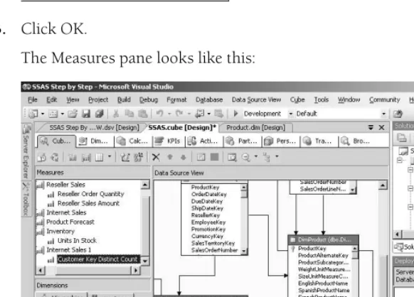
Suppose you decide to design a cube before you create the data warehouse to support it— which, incidentally, you can do in Analysis Services 2005. First, you select a measure—say, Sales Amount. Next, decide what dimensions you would like for that measure, and at what level of detail—say, Product by Customer, by Date. This defines the grain for the measure. Finally, decide if there are any other measures that have the same grain—perhaps Sales Units. You would then create a measure group that contains all the measures that have the same dimensions at the same grain.
A measure group is simply the group of measures that share the same grain. When you go to build your data warehouse, you would create a separate fact table for each measure group. Conversely, if you already have a data warehouse with several fact tables, you simply create a measure group for each fact table.
A cube is then the combination of all the measure groups. This means that a single cube can contain measures with different grains. This pushes the meaning of cube even further from its geometrical origins. Perhaps you can visualize a cube as a cluster of crystals of varying sizes and shapes, many of which share common sides. In this new way of thinking, a single cube can contain all the metadata for all the data in your data warehouse. Because of this, a cube is now sometimes called a Unified Dimensional Model, or UDM. Sometimes a cube has more information than is manageable by a single person. For example, a procurement manager may not care about how sales discounts are applied. Analysis Services allows you to create a per -spective that is like a cube that contains only a subset of the measures and dimensions of the whole cube. You can create as many perspectives as you want within a cube.
A cube is a logical structure, not a physical one. The same is true for a measure group. It defines the metadata so that client tools can access the data. You define measures and dimen-sions, and specify how measures should be aggregated across the dimensions.
Conceptually, each measure group contains all the detail values stored in the fact table, but that doesn’t mean that the measure group must physically copy all the detail values from the fact table. If you choose, you can make the measure group dynamically retrieve values as needed from the fact table. In this case, you’re using the measure group only to define meta-data. This is called relational OLAP, or ROLAP. For faster query performance, you can tell the measure group to copy the detail values into a proprietary structure that allows for extremely fast retrieval. This is called multidimensional OLAP, or MOLAP. Analysis Services allows you, as the cube designer, to decide whether to store the values as MOLAP or ROLAP. Aside from performance differences, where the detail values are physically stored is completely invisible to a user of a cube. Whether you use MOLAP or ROLAP, values are stored in a memory cache— on a space-available basis—to make subsequent queries faster. You can think of MOLAP stor-age as a disk-based cache that allows the Analysis Server to load the memory cache much faster than if it had to go to the relational database.