of generalized Lagrange spaces
M.I. Wanas, Nabil L. Youssef and A.M. Sid-Ahmed
Abstract. In this paper, we deal with a generalization of the geometry of parallelizable manifolds, or the absolute parallelism (AP-) geometry, in the context of generalized Lagrange spaces. All geometric objects de-fined in this geometry are not only functions of the positional argumentx, but also depend on the directional argumenty. In other words, instead of dealing with geometric objects defined on the manifoldM, as in the case of classical AP-geometry, we are dealing with geometric objects in the pullback bundle π−1(T M) (the pullback of the tangent bundle T M by
π:T M −→M). Many new geometric objects, which have no counterpart in the classical AP-geometry, emerge in this more general context. We refer to such a geometry as generalized AP-geometry (GAP-geometry). In analogy to AP-geometry, we define ad-connection inπ−1(T M) having
remarkable properties, which we call the canonicald-connection, in terms of the unique torsion-free Riemanniand-connection. In addition to these two d-connections, two more d-connections are defined, the dual and the symmetric d-connections. Our space, therefore, admits twelve curvature tensors (corresponding to the four definedd-connections), three of which vanish identically. Simple formulae for the nine non-vanishing curvatures tensors are obtained, in terms of the torsion tensors of the canonical d-connection. The differentW-tensors admitted by the space are also calcu-lated. All contractions of theh- andv-curvature tensors and theW-tensors are derived. Second rank symmetric and skew-symmetric tensors, which prove useful in physical applications, are singled out.
M.S.C. 2000: 53B40, 53A40, 53B50
Key words: Parallelizable manifold, Generalized Lagrange space, AP-geometry, GAP-geometry, Canonicald-connection,W-tensor.
∗
Balkan Journal of Geometry and Its Applications, Vol.13, No.2, 2008, pp. 120-139. c
1
Introduction
The geometry of parallelizable manifolds or the absolute parallelism geometry (AP-geometry) ([5], [10], [14], [15]) has many advantages in comparison to Riemannian geometry. Unlike Riemannian geometry, which has ten degrees of freedom (corre-sponding to the metric components forn= 4), AP-geometry has sixteen degrees of freedom (corresponding to the number of components of the four vector fields defin-ing the parallelization). This makes AP-geometry a potential candidate for describdefin-ing physical phenomena other than gravity. Moreover, as opposed to Riemannian geome-try, which admits only one symmetric linear connection, AP-geometry admits at least four natural (built-in) linear connections, two of which are non-symmetric and three of which have non-vanishing curvature tensors. Last, but not least, associated with an space, there is a Riemannian structure defined in a natural way. Thus, AP-geometry contains within its geometrical structure all the mathematical machinery of Riemannian geometry. Accordingly, a comparison between the results obtained in the context of AP-geometry and general relativity, which is based on Riemannian geometry, can be carried out.
In this paper, we study AP-geometry in the wider context of a generalized La-grange space ([7], [9], [11], [12]). All geometric objects defined in this space are not only functions of the positional argumentx, but also depend on the directional argument y. In other words, instead of dealing with geometric objects defined on the manifold M, as in the case of classical AP-space, we are dealing with geometric objects in the pullback bundleπ−1(T M) (the pullback of the tangent bundleT M by the projection π:T M −→M) [1]. Many new geometric objects, which have no counterpart in the classical AP-space, emerge in this more general context. We refer to such a space as ad-parallelizable manifold or a generalized absolute parallelism space (GAP-space).
The paper is organized in the following manner. In section 2, following the in-troduction, we give a brief account of the basic concepts and definitions that will be needed in the sequel, introducing the notion of a non-linear connection Nα
µ. In
section 3, we consider an n-dimensional d-parallelizable manifold M ([2], [11]) on which we define a metric in terms of thenindependentπ-vector fields
i
λdefining the parallelization onπ−1(T M). Thus, our parallelizable manifold becomes a generalized Lagrange space, which is a generalization of the classical AP-space. We then define the canonicald-connectionD, relative to which the h- and v-covariant derivatives of the vector fields
i
of the differentW-tensors and the relations between them are then derived. Finally, we end this paper by some concluding remarks.
2
Fundamental preliminaries
LetM be a differential manifold of dimension nof class C∞. Letπ: T M →M be its tangent bundle. If (U, xµ) is a local chart on M, then (π−1(U), (xµ, yµ)) is the
corresponding local chart onT M. The coordinate transformation law onT M is given by:
xµ′ =xµ′(xν), yµ′ =pµ′ ν yν,
wherepµ′ ν = ∂x
µ′
∂xν and det(pµ
′ ν )6= 0.
Definition 2.1. A non-linear connection N on T M is a system of n2 functions
Nα
β(x, y) defined on every local chartπ−1(U) of TM which have the transformation
law
(2.1) Nβα′′ =pα ′ αp
β
β′Nβα+pα ′ ǫ pǫβ′σ′yσ
′
,
wherepǫβ′σ′ = ∂pǫ
β′
∂xσ′ =
∂2xǫ
∂xβ′∂xσ′.
The non-linear connectionN leads to the direct sum decomposition
Tu(T M) =Hu(T M)⊕Vu(T M), ∀u∈ TM =T M\ {0},
whereHu(T M) is thehorizontalspace atuassociated withN supplementary to the
verticalspaceVu(T M). Ifδµ:=∂µ−Nµα∂˙α, where∂µ :=∂x∂µ, ˙∂µ:=∂y∂µ, then ( ˙∂µ) is
the natural basis ofVu(T M) and (δµ) is the natural basis ofHu(T M) adapted toN.
Definition 2.2. A distinguished connection (d-connection) on M is a triplet D = (Nα
µ,Γαµν, Cµνα), whereNµα(x, y) is a non-linear connection on T M and Γαµν(x, y) and
Cα
µν(x, y) transform according to the following laws:
(2.2) Γαµ′′ν′ =pα ′ αp
µ
µ′pνν′Γαµν+pα ′ ǫ pǫµ′ν′,
(2.3) Cµα′′ν′ =pα ′ αp
µ
µ′pνν′Cµνα .
In other words, Γα
µν transform as the coefficients of a linear connection, whereasCµνα
transform as the components of a tensor.
Definition 2.3. The horizontal (h-) and vertical (v-) covariant derivatives with re-spect to the d-connectionD (of a tensor fieldAα
µ) are defined respectively by:
(2.4) Aαµ|ν:=δνAαµ+AǫµΓαǫν−AαǫΓǫµν;
Definition 2.4. A symmetric and non-degenerate tensor fieldgµν(x, y) of type (0, 2)
is called a generalized Lagrange metric on the manifoldM. The pair (M, g) is called a generalized Lagrange space.
Definition 2.5. Let (M, g) be a generalized Lagrange space equipped with a non-linear connectionNα
µ. Then a d -connectionD= (Nµα,Γαµ,ν, Cµνα ) is said to be metrical
with respect tog if
(2.6) gµν|α= 0, gµν||α= 0.
The following remarkable result was proved by R. Miron [8]. It guarantees the existence of a uniquetorsion-freemetricald-connection on any generalized Lagrange space equipped with a non-linear connection. More precisely:
Theorem 2.6. Let (M, g) be a generalized Lagrange space. LetNα
µ be a given
non-linear connection on T M. Then there exists a unique metrical d-connection
◦ d-connection is given by Nα
µ and the generalized Christoffel symbols:
(2.7)
This connection will be referred to as the Riemanniand-connection.
3
d
-Parallelizable manifolds (GAP-spaces)
The Riemannian d-connection mentioned in Theorem 2.6 plays the key role in our generalization of the AP-space, which, as will be revealed, appears natural. However, it is to be noted that the close resemblance of the two spaces is deceptive; as they are similar in form. However, the extra degrees of freedom in the generalized AP-space makes it richer in content and different in its geometric structure (see Remark 3.6).
We start with the concept ofd-parallelizable manifolds.
Definition 3.1. Ann-dimensional manifoldM is called d-parallelizable, or general-ized absolute parallelism space (GAP-space), if the pull-back bundleπ−1(T M) admits nglobal linearly independent sections (π-vector fields)
i
Einstein summation convention is applied on both Latin (mesh) indices and Greek (world) indices, where all Latin indices are written in a lower position.
In the sequel, we will simply use the symbolλ(without a mesh index) to denote any one of the vector fields
i
We shall often use the expression GAP-space (resp. GAP-geometry) instead of d-parallelizable manifold (resp. geometry of d-parallelizable manifolds) for its typo-graphical simplicity.
Theorem 3.2. A GAP-space is a generalized Lagrange space.
In fact, the covariant tensor fieldgµν(x, y) of order 2 given by
(3.2) gµν(x, y) :=
i
λµ
i
λν,
defines a metric in the pull-back bundleπ−1(T M) with inverse given by
(3.3) gµν(x, y) =
i
λµ
i
λν
Assume thatM is a GAP-space equipped with a non-linear connection Nα µ. By
Theorem 2.6, there exists on (M, g) a unique torsion-free metricald-connection
◦
Cαµν) (the Riemanniand-connection). We define another d-connectionD= (Nα with respect to thed-connectionD, then
(3.6) λα|µ= 0, λα||µ= 0.
λ(x, y)) be a GAP-space equipped with a non-linear con-nection Nα
µ. There exists a unique d-connection D = (Nµα,Γαµν, Cµνα), such that
λα
|µ = λα||µ = 0. This connection is given by Nβα, (3.4) and (3.5). Consequently,
D is metrical:gµν|σgµν||σ= 0.
This connection will be referred to as the canonicald-connection.
It is to be noted that relations (3.6) are in accordance with the classical AP-geometry in which the covariant derivative of the vector fieldsλwith respect to the canonical connection Γα
λ(x, y)) be a d-parallelizable manifold equipped with a non-linear connection Nµα. The canonical d-connection D = (Nα
µ,Γαµν, Cµνα ) is explicitly
expressed in terms of λin the form
Proof. Since λα
|ν = 0, we haveδνλα=−λǫΓαǫν. Multiplying both sides byλµ, taking
into account the fact that
i
proof of the second relation is exactly similar and we omit it.
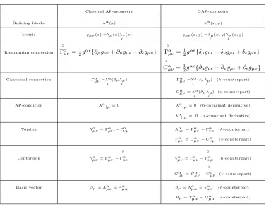
It is to be noted that the components of the canonical d-connection are similar in form to the components of the canonical connection in the classical AP-context [15], noting that ∂ν is replaced by δν (for the h-counterpart) and by ˙∂ν (for the
v-counterpart) respectively (See Table 1). The above expressions for the canonical connection seem therefore like a natural generalization of the classical AP case.
By (3.4) and (3.5), in view of the above theorem, we have the following Corollary 3.5. The Reimannian d-connection
◦
A◦. s a result of the dependence of λ on the velocity vector y, the n3 functions
i
λα(∂ν
i
λµ), as opposed to the classical AP-space, do not transform as the coefficients
of a linear connection, but transform according to the rule (3.9)
Similarly, it can be shown that, in general, tensors in the context of the classical AP-space do not transform like tensors in the wider context of the GAP-space; their dependence on the velocity vector y spoils their tensor character. In other words, tensors in the classical AP-context do not necessarily behave like tensorswhen they are regarded as functions of positionxand velocity vectory.This means that though the classical AP-space and the GAP-space appear similar in form, they differ radically in their geometric structures. We now introduce some tensors that will prove useful later on. Let In analogy to the AP-space, we refer toγα
µν andGαµνas theh- andv-contortion tensors
respectively. Let
(3.11) Λα
µν := Γαµν−Γανµ=γµνα −γνµα .
be the torsion tensor of the canonical connection Γα µν and
(3.12) Ωαµν :=γµνα +γνµα .
Similarly, let
(3.13) Tµνα :=Cµνα −Cνµα =Gαµν−Gανµ be what we may call the torsion tensor ofCα
µν and
(3.14) Dαµν :=Gαµν+Gανµ.
Now, ifγσµν:=gǫσγǫµν andGσµν:=gǫσGǫµν, thenγσµνandGσµνare skew symmetric
Table 1. Comparison between the classical AP-geometry
Canonical connection Γαµν=
i
Finally, it can be shown, in analogy to the classical AP-space [3], that the contor-tion tensors γµνσ and Gµνσ can be expressed in terms of the torsion tensors in the
form
(3.18) that the torsion tensors vanish if and only if the contortion tensors vanish.
Table 1 gives a comparison between the fundamental geometric objects in the classical AP-geometry and the GAP-geometry. Similar objects of the two spaces will be denoted by the same symbol. As previously mentioned, “h” stands for “horizontal” whereas “v” stands for “vertical”.
4
Curvature tensors in Generalized AP-space
Lemma 4.1. Let[δσ, δµ] :=δσδµ−δµδσ and let[δσ,∂˙µ]be similarly defined. Then
(4.1) [δσ, δµ] =Rǫσµ∂˙ǫ, [δσ,∂˙µ] = ( ˙∂µNσǫ) ˙∂ǫ,
whereRα
σµ:=δµNσα−δσNµαis the curvature tensor of the non-linear connectionNµα.
Theorem 4.2. The three commutation formulae of
i
λαcorresponding to the canonical connectionD= (Nα
µ,Γαµν, Cµνα) are given by
(a) λα
|µσ−λα|σµ=λǫRǫµσα +λα|ǫΛǫσµ+λα||ǫRǫσµ
(b) λα
||µσ−λα||σµ=λǫSǫµσα +λα||ǫTσµǫ
(c) λα
||µ|σ−λα|σ||µ=λǫPǫµσα +λα|ǫCσµǫ + λα||ǫPσµǫ ,
where
Rανµσ: = (δσΓανµ−δµΓανσ) + (Γνµǫ Γαǫσ−ΓǫνσΓαǫµ) +Lανµσ, (h-curvature)
Sνµσα : = ˙∂σCνµα −∂˙µCνσα +Cνµǫ Cǫσα −Cνσǫ Cǫµα, (v-curvature)
Pνµσα : = Cνµα|σ−∂˙µΓανσ−Pσµǫ Cνǫα, (hv-curvature)
given that Lα
νµσ:=CνǫαRǫµσ and Pσµν := ˙∂µNσν−Γνµσ.
A direct consequence of the above commutation formulae, together with the fact that λα
|µ=λα||µ= 0,is the following
Corollary 4.3. The three curvature tensors Rα
νµσ, Sνµσα and Pνµσα of the canonical
connectionD= (Nα
µ,Γαµν, Cµνα) vanish identically.
It is to be noted that the above result is a natural generalization of the corre-sponding result of the classical AP-geometry [15].
The Bianchi identities [4] for the canonicald-connection (Nα
µ,Γαµν, Cµνα) gives
Proposition 4.4. The following identities hold
(a) Sν,µ,σΛα
νµ|σ =Sν,µ,σ(ΛµǫαΛǫνσ+Lαµνσ)
(b) Sν,µ,σTα
νµ||σ=Sν,µ,σ(TµǫαTνσǫ ),
whereSν,µ,σ denotes a cyclic permutation on ν, µ, σ.
Corollary 4.5. The following identities hold:
(a) Λǫ
µν|ǫ=βµ|ν−βν|µ+βǫΛǫµν+Sǫ,ν,µLǫǫνµ.
(b) Tǫ
µν||ǫ=Bµ||ν−Bν||µ+BǫTµνǫ ,
Proof. Both identities follow by contracting the indices α and σ in the identities (a) and (b) of Proposition 4.4, taking into account that βµ = Λǫµǫ, Bµ = Tµǫǫ and
Lα
In addition to the Riemannian and the canonicald-connections, our space admits at least two other natural d-connections. In analogy to the classical AP-space, we define the duald-connectionDe = (Nα
µ,Γeαµν,Ceµνα ) by
(4.2) Γeα
µν := Γανµ, Ceµνα :=Cνµα
and the symmetricd−connectionDb = (Nα
µ,bΓαµν,Cbµνα ) by
(4.3) Γbαµν :=
1 2(Γ
α
µν+ Γανµ), Cbµνα :=
1 2(C
α
µν+Cνµα).
Covariant differentiation with respect toΓeα
µν andbΓαµν will be denoted by “e|” and “b|”
respectively.
Now, corresonding to each of the fourd-connections there are three curvature ten-sors. Therefore, we have a total of twelve curvature tensors three of which, as already mentioned, vanish identically. The vanishing of the curvature tensors of the canoni-cald-connection allows us to express, in a relatively compact form, six of the other curvature tensors (theh- andv-curvature tensors) corresponding to the Riemannian, symmetric and the duald-connections. These curvature tensors are expressed in terms of the torsion tensors Λα
µν, Tµνα and their covariant derivatives with respect to the
canonicald-connection, together with the curvatureRα
µν of the non-linear connection
Nα
µ.The other threehv-curvature tensors are calculated, though their expressions are
more complicated. This is to be expected since the expression obtained for the hv-curvature tensor of the canonicald-connection lacks the symmetry properties enjoyed by theh- andv-curvature tensors.
Theorem 4.6. The h-, v- and hv-curvature tensors of the dual d-connection De = (Nα
µ,Γeαµν,Ceµνα)can be expressed in the form:
(a) Reα
µσν= Λασν|µ+CǫµαRǫσν+Lασνµ+Lανµσ.
(b) Seµσνα =Tσνα||µ.
(c) Peα
νµσ=Tµνα|σ−Λσνα ||µ+Tµνǫ Λασǫ−TµǫαΛǫσν−ΛαǫνCσµǫ −Pσµǫ Tǫνα.
The corresponding curvature tensors of the symmetric d-connectionDb = (Nα
µ,Γbαµν,Cbµνα)
can be expressed in the form:
(d) Rbα
µσν= 12(Λαµν|σ−Λαµσ|ν) +
1
4(ΛǫµνΛασǫ−ΛǫµσΛανǫ) +21(ΛǫσνΛαǫµ) +12(TǫµαRǫσν).
(e) Sbα
µσν =12(Tµνα||σ−Tµσα||ν) +
1
4(Tµνǫ Tσǫα −Tµσǫ Tνǫα) +12(Tσνǫ Tǫµα).
(f ) Pbα
νµσ= 12 (Λαµν|σ−Λασν||µ) +
1
4 ΛǫσµTǫνα−12 ΛαǫνCσµǫ +41 Sµ,ν,σΛǫµνΛασǫ−12 Pσµǫ Tǫνα.
The corresponding curvature tensors of the Riemannian d-connection
◦
D= (Nα µ,
◦
Γαµν, ◦
Cαµν) can be expressed in the form
(g)
◦
Rαµσν=γα
(h)
◦
Sαµσν=Gαµν||σ−Gαµσ||ν+Gµσǫ Gαǫν−GǫµνGαǫσ+GαµǫTνσǫ .
(i)
◦
Pανµσ= ˙∂uγνσα −Gανµ|σ+ (Gǫνµ−Cνµǫ )γǫσα −(Gαǫµ−Cǫµα)γνσǫ +Pσµǫ Gανǫ.
Proof. We prove (a) and (c) only. The proof of the other parts is similar.
(a) We have
e
Rαµσν = δνeΓαµσ−δσΓeαµν+eΓµσǫ Γeαǫν−ΓeǫµνΓeαǫσ+CeµǫαRǫσν
= δνΓασµ−δσΓανµ+ ΓǫσµΓανǫ−ΓǫνµΓασǫ+CǫµαRǫσν
= {δνΓασµ+ Γǫσµ(Λανǫ+ Γαǫν)} − {δσΓανµ+ Γǫνµ(Λασǫ+ Γαǫσ)}
+CǫµαRǫσν
= (δνΓασµ+ ΓǫσµΓαǫν)−(δσΓανµ+ ΓǫνµΓαǫσ)−(ΓǫσµΛαǫν+ ΓǫνµΛασǫ)
+Cα ǫµRǫσν
= (Rα
σµν−CσǫαRǫµν+δµΓασν+ Γσνǫ Γαǫµ)−(Rανµσ−CνǫαRǫµσ
+δµΓανσ+ Γνσǫ Γαǫµ)−(ΓǫσµΛαǫν+ ΓǫνµΛασǫ) +CǫµαRǫσν.
= δµΛασν+ ΓαǫµΛσνǫ −ΓǫσµΛαǫν−ΓǫνµΛασǫ+CǫµαRǫσν+CσǫαRǫνµ+CνǫαRǫµσ
= Λασν|µ+CǫµαRǫσν+Lασνµ+Lανµσ.
(c) We have
e
Pνµσα = Cµναe|σ−∂˙µΓ α
σν−( ˙∂µNσǫ−Γǫσµ)Cǫνα
= Cνµα|σ+ (Cµναe|σ−Cνµα|σ)−∂˙µΛασν−∂˙µΓανσ−∂˙µNσǫ(Tǫνα +Cνǫα)
+ (Λǫσµ+ Γǫµσ)(Tǫνα +Cνǫα)
= Pνµσα −( ˙∂µNσǫ−Γǫµσ)Tǫνα −∂˙µΛασν+ ΛǫσµCǫνα + (Cµναe|σ−C α νµ|σ)
= (Cα
µνe|σ−C α νµ|σ) + Λ
ǫ
σµCǫνα −∂˙µΛασν−Pσµǫ Tǫνα
= Tµνα|σ+Cµνǫ Λα
σǫ−CµǫαΛǫσν−∂˙µΛασν−Pσµǫ Tǫνα
= Tµνα|σ−∂˙µΛασν+ (Tµνǫ +Cνµǫ )Λασǫ−(Tµǫα +Cǫµα)Λǫσν−Pσµǫ Tǫνα
= Tµνα|σ−Λα
σν||µ+Tµνǫ Λασǫ−TµǫαΛσνǫ −ΛαǫνCσµǫ −Pσµǫ Tǫνα.
which are the required formulae.
5
Fundamental second rank tensors
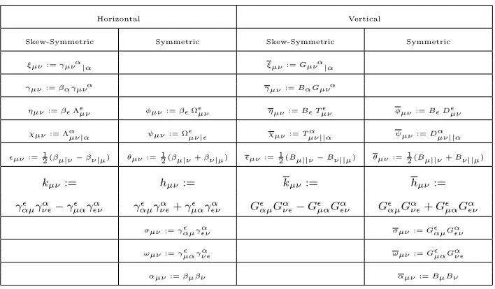
and “vertical” tensors are denoted by the same symbol with the “vertical” tensors barred. It is to be noted that all “vertical ” tensors have no counterpart in the classical AP-context.
Table 2. Summary of the fundamental symmetric and skew-symmetric second rank tensors
Horizontal Vertical
Skew-Symmetric Symmetric Skew-Symmetric Symmetric
ξµν:=γµνα|α ξµν:=Gµνα|α
γµν:=βαγµνα γµν:=BαGµνα
ηµν:=βǫΛǫµν φµν:=βǫΩµνǫ ηµν:=Bǫ Tµνǫ φµν:=Bǫ Dǫµν
χµν:= Λαµν|α ψµν:= Ωǫµν|ǫ χµν:=T αµν||α ψµν:=Dαµν||α
ǫµν:= 12(βµ|ν−βν|µ) θµν:= 12(βµ|ν+βν|µ) ǫµν:= 12(Bµ||ν−Bν||µ) θµν:= 12(Bµ||ν+Bν||µ)
kµν := hµν:= kµν:= hµν :=
γǫ αµγ
α ν ǫ−γ
ǫ µαγ
α ǫν γ
ǫ αµγ
α ν ǫ+γ
ǫ µαγ
α ǫν G
ǫ αµG
α ν ǫ−G
ǫ µαG
α ǫν G
ǫ αµG
α ν ǫ+G
ǫ µαG
α ǫν
σµν:=γǫαµ γαǫν σµν:=Gǫαµ Gαǫν
ωµν:=γǫµα γνǫα ωµν:=Gǫµα Gανǫ
αµν:=βµβν αµν:=BµBν
Due to the metricity condition in Theorem 3.3, one can use the metric tensorgµν
and its inversegµν to perform the operations of lowering and raising tensor indices
under theh- andv- covariant derivatives relative to the canonicald-connection. Thus, contraction with the metric tensor of the above fundamental tensors gives the following table of scalars:
Table 3. Summary of the fundamental scalars
Horizontal α:=βµβµ θ:=βµ|µ φ:=βǫΩǫµµ ψ:= Ωαµµ|α
ω:=γǫµ
αγαµǫ σ:=γ ǫ
αµγǫµα h:= 2γ αµ
ǫγǫαµ
Vertical α:=BµBµ θ:=Bµ|µ φ:=BǫDǫµµ ψ:=Dαµµ|α
ω:=Gǫµ
αGαµǫ σ:=G ǫ
αµGαǫµ h:= 2G αµ
ǫGǫαµ
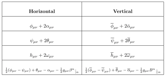
Table 4. Summary of the fundamental tensors of zero trace
Horizontal Vertical
φµν+ 2αµν φµν+ 2 ¯αµν
ψµν+ 2θµν ψµν+ 2θµν
hµν+ 2ωµν hµν+ 2ωµν
1
2(φµν−ψµν) +θµν−αµν−12gµνβαe|α
1
2(φµν−ψµν) +θµν−αµν−12gµνBαe||α
We now consider some useful second rank tensors which are not expressible in terms of the fundamental tensors appearing in Table 2. Unlike the tensors of Table 2, some of the tensors to be defined below have no horizontal and vertical counterparts. To this end, let
Lµν :=Lααµν=CαǫαRǫµν, Mµν :=Lαµαν =Cµǫα Rǫαν, Nµν :=Cǫµα Rǫαν, Fµν := ◦
CαǫµRǫαν.
Then, clearly
Tµν :=Mµν−Nµν =Tµǫα Rǫαν, Gµν :=Mµν−Fµν =GαµǫRǫαν, Gµν−Tµν =GαǫµRǫαν.
Finally, let T :=gµνT
µν and G:=gµνGµν. By the above, we have the following:
Symmetric second rank tensors:M(µν), N(µν), F(µν).
Skew-symmetric second rank tensors:M[µν], N[µν], F[µν], Lµν.
6
Contracted curvatures and curvature scalars
It may be convenient, for physical reasons, to consider second rank tensors derived from the curvature tensors by contractions. It is also of interest to reduce the number of these tensors to a minimum which is fundamental (cf. Propositions 6.1 and 6.2).
Contracting the indices α and µ in the expressions obtained for the h- and v-curvature tensors in Theorem 4.6, taking into account Corollary 4.5, we obtain
Proposition 6.1. Let Reσν :=Reαασν, Rbσν :=Rbαασν and ◦
Rσν := ◦
Rαασν with similar
expressions forSeσν,Sbσν and ◦
Sσν. Then, we have
(a) Reσν =βσ|ν−βν|σ+βǫΛǫσν+BǫRǫσν,
(b) Seσν =Bσ||ν−Bν||σ+BǫTσνǫ ,
(c) Rbσν =12Reσν,
(e)
◦
Rσν = ◦
Sσν = 0.
Proposition 6.2. Let Reµσ :=Reαµσα, Rbµσ :=Rbµσαα and ◦
Rµσ := ◦
Rαµσα with similar
expressions forSeµσ,Sbµσ and ◦
Sµσ. Then, we have
(a) Reµσ =βσ|µ+CǫµαRǫσα+Lασαµ+Lααµσ,
(b) Seµσ =Bσ||µ,
(c) Rbµσ =12Reµσ+14{βǫΛǫσµ+ ΛǫασΛαµǫ},
(d) Sbµσ =12Seµσ+14{BǫTσµǫ +Tασǫ Tµǫα},
(e)
◦
Rµσ=βµ|σ−γµσα |α+βǫγ ǫ
µσ−γµǫαγσαǫ +GαµǫRǫασ,
(f )
◦
Sµσ := ◦
Sαµσα=Bµ||σ−Gαµσ||α+BǫGǫµσ−GαµǫGǫσα.
Proposition 6.3. The following holds.
(a) Re[µσ]= 12{βσ|µ−βµ|σ}+Cǫαǫ Rαµσ+C(ǫασ)Rαǫµ−C(ǫαµ)Rǫσα,
(b) Re(µσ)= 21{βσ|µ+βµ|σ+Tαµǫ Rασǫ+Tασǫ Rαµǫ},
(c) Se[µσ]= 12{Bσ||µ−Bµ||σ},
(d) Se(µσ)=12{Bσ||µ+Bµ||σ},
(e) Rb[µσ]=12Re[µσ]+14βǫΛǫσµ,
(f ) Rb(µσ)= 12Re(µσ)+14ΛǫασΛαµǫ,
(g) Sb[µσ]= 12Se[µσ]+14BǫTσµǫ ,
(h) Sb(µσ)=12Se(µσ)+14Tασǫ Tµǫα,
(i)
◦
R[µσ] =12{Lααµσ+ ◦
CασǫRǫ αµ−
◦
CαµǫRǫ ασ},
(j)
◦
R(µσ)=12{(βµ|σ+βσ|µ)−Ωαµσ|α+βǫΩǫµσ} −γµǫα γσαǫ +12{GαµǫRǫασ+GασǫRǫαµ},
(k)
◦
S[µσ]= 0,
(l)
◦
S(µσ)=12{(Bµ||σ+Bσ||µ)−Dαµσ||α+BǫDµσǫ } −GαµǫGǫσα.
Corollary 6.4. The following holds:
(a) Reσ
σ:=gµσReµσ=βσ|σ+TǫσαRαǫσ,
(b) Seσ
(c) Rbσ
We now apply a different method for calculating both
◦
Rµσand ◦
Sµσ, now expressed
in terms of the covariant derivative of the contorsion tensors with respect to the Riemanniand-connection. Then we obtain
Proposition 6.5. The “Ricci” tensors
◦
Rµσ and ◦
Sµσ can be expressed in the form
(a)
Proof. We prove(a)only; the proof of(b)is similar. We have
which is the required formula.
In view of Proposition 6.2 (e) and (f) and Proposition 6.5, we obtain
Corollary 6.6. The following identities holds:
(a) (βµ|σ−βµo
Table 5 (a). Second rank curvature tensors
Skew-symmetric Symmetric
Dual Re[µσ]=ǫσµ−Lσµ+M[σµ]+N[σµ] Re(µσ)=θµσ+M(µσ)−N(µσ)
e
S[µσ]=ǫσµ Se(µσ)=θµσ
Symmetric Rb[µσ]=12Re[µσ]+14ησµ Rb(µσ)=
1 2Re(µσ)+
1
4{hµσ−ωµσ−σµσ}
b
S[µσ]=12Se[µσ]+14ησµ Sb(µσ)= 12Se(µσ)+41{hµσ−ωµσ−σµσ}
Riemannian
◦ R[µσ]=
1
2Lµσ−F[µσ]
◦
R(µσ)=θµσ−
1
2(ψµσ−φµσ)
−ωµσ+M(µσ)−F(µσ)
◦ S[µσ]= 0
◦
S(µσ)=θµσ−
1
2(ψµσ−φµσ)−ωµσ
Table 5 (b). h- and v-scalar curvature tensors
h-scalar curvature v-scalar curvature
Dual Reσ
σ=θ+T Seσσ=θ
Symmetric Rbσ
σ=12(θ+T)− 1
4(3ω+σ) Sbσσ= 12θ− 1
4(3ω+σ)
Riemannian
◦
Rσσ=θ−12(ψ−φ)−ω+G
◦
Sσσ=θ−12(ψ−φ)−ω
7
The
W
-tensors
The W-tensor was first defined by M. Wanas in 1975 [13] and has been used by F. Mikhail and M. Wanas [6] to construct a geometric theory unifying gravity and electromagnetism. Recently, two of the authors of this paper studied some of the properties of this tensor in the context of the classical AP-space [15].
Definition 7.1. Let (M, λ) be a generalized AP-space. For a given d-connection D = (Nα
β,Γαµν, Cµνα ), the horizontal W-tensor (hW-tensor) Hµνσα is defined by the
formula
λµ|νσ−λµ|σν =λǫHµνσǫ ,
whereas the verticalW-tensor (vW-tensor)Vµνσα is defined by the formula
λµ||νσ−λµ||σν=λǫVµνσǫ ,
We now carry out the task of calculating the differentW-tensors. As opposed to the classical AP-space, which admits essentially oneW-tensor corresponding to the dual connection, we here have 4 distinctW-tensors: the horizontal and verticalW-tensors corresponding to the duald-connection, the horizontalW-tensor corresponding to the symmetric d-connection and, finally, the horizontal W-tensor corresponding to the Riemanniand-connection. The remainingW-tensors coincide with the corresponding curvature tensors.
It is to be noted that some of the expressions obtained for the W-tensors are relatively more compact than those obtained for the corresponding curvature tensors.
Theorem 7.2. The hW-tensor Heα
µνσ, the vW-tensorVeµνσα , the hW-tensorHbµνσα and
the hW-tensor
◦
Hαµνσ corresponding to the dual, symmetric and the Riemannian d-connections respectively can be expressed in the form:
(a) Heµνσα = Λα σν|µ+ Λ
ǫ
νσΛαµǫ+Sµ,ν,σLαµσν.
(b) Veα
µνσ=Tσνα||µ+Tνσǫ Tµǫα.
(c) Hbα
µνσ =12(Λαµν|σ−Λαµσ|ν) +
1
4(ΛǫµνΛασǫ−ΛǫµσΛανǫ) +12(ΛǫσνΛαǫµ).
(d)
◦
Hαµνσ=γα
µν|σ−γαµσ|ν+γµσǫ γǫνα −γǫµνγǫσα + Λǫνσγµǫα.
Proof. We prove(a)only. The proof of the other parts is similar. We have
λǫHeµνσǫ =λǫReǫµσν+λµe|ǫΛe ǫ
σν+λµe||ǫR ǫ σν.
Hence, taking into account Theorem 4.6 (a), we obtain
e
Hµνσα = Reαµσν+
i
λα(δǫ
i
λµ−
i
λβΓβǫµ)Λeǫσν+λiα( ˙∂ǫ
i
λµ−
i
λβCǫµβ)Rǫσν
= Reαµσν+ Λǫ
νσ(Γαµǫ−Γαǫµ) +Rσνǫ (Cµǫα −Cǫµα)
= Λασν|µ+CǫµαRǫσν+Lασνµ+Lανµσ+ ΛǫνσΛαµǫ+TµǫαRσνǫ
= Λα
σν|µ+TǫµαRσνǫ +CµǫαRǫσν+Lασνµ+Lανµσ+ ΛǫνσΛαµǫ+ TµǫαRǫσν
= Λα
σν|µ+ ΛǫνσΛαµǫ+Sµ,ν,σLαµσν.
Proposition 7.3. Let Heνσ :=Heανσα ,Hbνσ :=Hbανσα and ◦
Hνσ := ◦
Hαανσ with similar expression forVeνσ. Then, we have
(a) Heνσ=βσ|ν−βν|σ+ 2βǫΛǫσν,
(b) Veνσ=Bσ||ν−Bν||σ+ 2BǫTσνǫ ,
(c) Hbνσ=12{Heνσ+βǫΛǫνσ},
(d)
◦
Proposition 7.4. Let Heµσ :=Heµασα ,Hbµσ :=Hbµασα and ◦
Hµσ := ◦
Hαµασ with similar expressions forVeµσ. Then, we have
(a) Heµσ =βσ|µ+ Λασǫ Λαµǫ+Sα,µ,σLααµσ,
(b) Veµσ=Bσ||µ+Tασǫ Tµǫα,
(c) Hbµσ =12Heµσ+41(βǫΛǫσµ+ ΛǫσαΛαµǫ),
(d)
◦
Hµσ =βµ|σ−γµσα|α+βǫγµσǫ −γσαǫ γαµǫ.
Proposition 7.5. The following holds:
(a) He[µσ]= 12{βσ|µ−βµ|σ}+Sα,µ,σLααµσ,
(b) He(µσ)= 12{βσ|µ+βµ|σ}+ ΛǫασΛαµǫ,
(c) Ve[µσ]= 12{Bσ||µ−Bµ||σ},
(d) Ve(µσ)= 12{Bσ||µ+Bµ||σ}+Tασǫ Tµǫα,
(e) Hb[µσ]=12He[µσ]+14βǫΛǫσµ,
(f ) Hb(µσ)= 12He(µσ)+14ΛǫσαΛαµǫ,
(g)
◦
H[µσ] =12SαµσLααµσ,
(h)
◦
H(µσ)= 12{(βµ|σ+βσ|µ)−Ωαµσ|α+βǫΩµσǫ } −γµǫαγσαǫ .
Corollary 7.6. the following holds:
(a) Heα
α =βα|α+ ΛǫµαΛαǫµ,
(b) Veα
α =Bα||α+TǫµαTǫµα,
(c) Hbα
α = 12βα|α+14ΛǫµαΛαǫµ,
(d)
◦
Hσσ=βσ|σ−12Ωασσ|α+12βαΩασσ−γασǫγσαǫ .
Taking into account Proposition 4.4, Theorem 7.2 and the Bianchi identity [4] for the Riemannian d-connection, we get the following
Proposition 7.7. The hW-tensors Heα
µνσ, Hbµνσα , ◦
Hαµνσ and the vW-tensors Veα µνσ
satisfy the following identities:
(a) Sµ,ν,σHeα
µνσ = 2Sµ,ν,σ(ΛαµǫΛǫνσ+Lαµσν).
(b) Sµ,ν,σVeα
µνσ= 2Sµ,ν,σ(TµǫαTνσǫ ).
(c) Sµ,ν,σHbα
(d) Sµ,ν,σ
◦
Hαµνσ=Sµ,ν,σLα
µσν.
We collect the results obtained in this section in the following tables, where the contractedW-tensors are expressed in terms of the fundamental tensors.
Table 6 (a). Second rank W-tensors
Skew-symmetric Symmetric
Dual He[µσ]=ǫσµ−Lσµ+ 2M[σµ] He(µσ)=θµσ−(ωµσ+σµσ−hµσ)
e
V[µσ]= ¯ǫσµ Ve(µσ)= ¯θµσ−(¯ωµσ+ ¯σµσ−¯hµσ)
Symmetric Hb[µσ]= 12He[µσ]+14ησµ Hb(µσ)= 12He(µσ)+14{ωµσ+σµσ−hµσ}
Riemannian
◦
H[µσ]= 12Lµσ−M[µσ]
◦
H(µσ)=θµσ−12(ψµσ−φµσ)−ωµσ
Table 6 (b). Scalar W-tensors
h-scalar W-tensors v-scalar W-tensors
Dual Heσ
σ =θ−(3ω+σ) Veσσ= ¯θ−(3¯ω+ ¯σ)
Symmetric Hbσ
σ = 12θ− 1
4(3ω+σ)
Riemannian
◦
Hσσ=θ−12(ψ−φ)−ω
Concluding remarks
On the present work, we have the following comments and remarks:
1. Existing theories of gravity suffer from some problems connected to recent ob-served astrophysical phenomena, especially those admitting anisotropic be-havior of the system concerned (e.g. the flatness of the rotation curves of spiral galaxies). So, theories in which the gravitational potential dependson both po-sition and directionare needed. Such theories are to be constructed in spaces admitting this dependence. This is one of the aims motivating the present work.
2. Among the advantages of the AP-geometry are the ease in calculations and the diverse and its thorough applications. In this work, we have kept as close as possible to the classical AP-case. However, the extra degrees of freedom in our GAP-geometry have created an abundance of geometric objects which have no counterpart in the classical AP-geometry. Since the physical meaning of most of the geometric objects of the classical AP-structure is clear, we hope to attribute physical meaning to the new geometric objects appearing in the present work, especially the vertical quantities.
3. Due to the wealth of the GAP-geometry, one is faced with the problem of choosing geometric objects that represent true physical quantities. As a first step to solve this problem, we have written all second order tensors in terms of the fundamental tensors defined in section 5. This is done to facilitate comparison between these tensors and to be able to choose the most appropriate for physical application. The same procedure has been used for scalars.
4. The paper is not intended to be an end in itself. In it, we try to construct a geometric framework capable of dealing with and describing physical phenom-ena. The success of the classical AP-geometry in physical applications made us choose this geometry as a guide line.
The physical interpretation of the geometric objects existing in the GAP-geometry and not in the AP-GAP-geometry will be further investigated in a forth-coming paper.
This paper is not an end in itself, but rather the beginning of a research direction. The physical interpretation of the geometric objects in the GAP-space that have no counterpart in the classical AP-space will be further investigated in forthcoming papers.
Acknowledgement.This paper was presented in “ The International Conference on Finsler Extensions of Relativity Theory” held at Cairo, Egypt, November 4-10, 2006. ArXiv Number: 0704.2001.
References
[1] D. Bao, S. Chern and Z. Shen, An introduction to Riemann-Finsler Geometry, Graduate Texts in Mathematics, Springer, 2000.
[3] K. Hayashi and T. Shirafuji, New general relativity, Phys. Rev. D 19 (1979), 3524-3554.
[4] M. Matsumoto,Foundations of Finsler Geometry and special Finsler spaces, Kai-seisha Press, Otsu, Japan, 1986.
[5] F. I. Mikhail, Tedrad vector fields and generalizing the theory of relativity, Ain Shams Sc. Bull., No. 6 (1962), 87-111.
[6] F. I. Mikhail and M.I Wanas,A generalized field theory. I. Field equations, Proc. R. Soc. London, A. 356 (1977), 471-481.
[7] R. Miron,A Lagrangian theory of relativity, Sem de Geom. si Top., 84, Timisoara, Romania, 1985.
[8] R. Miron,Metrical Finsler structures and special Finsler spaces, J. Math. Kyoto Univ., 23 (1983), 219-224.
[9] R. Miron,Compendium on the Geometry of Lagrange Spaces, Handbook of Dif-ferential Geometry, Vol. II (2006), 437-512.
[10] H. P. Robertson,Groups of motion in spaces admitting absolute parallelism, Ann. Math, Princeton (2), 33 (1932), 496 - 520.
[11] T. Sakaguchi,Parallelizable generalized Lagrange spaces, Anal. Sti. Univ. AI. I. Cuza, Iasi, Mat., 33, 2 (1987), 127-136.
[12] T. Sakaguchi,Invariant theory of parallelizable Lagrange spaces, Tensor, N. S., 46 (1987), 137-144.
[13] M. I. Wanas,A generalized field theory and its applications in cosmology, Ph. D. Thesis, Cairo University, 1975.
[14] M. I. Wanas, Absolute parallelism geometry: Developments, applications and problems, Stud. Cercet, Stiin. Ser. Mat. Univ. Bacau, No. 10 (2001), 297-309. [15] N. L. Youssef and A. M. Sid-Ahmed,Linear connections and curvature tensors
in the geometry of parallelizable manifolds, Submitted.
Authors’ addresses:
M. I. Wanas,
Cairo University, Faculty of Science, Department of Astronomy, Cairo, Egypt. E-mail: [email protected]
Nabil L. Youssef,
Cairo University, Faculty of Science, Department of Mathematics, Cairo, Egypt.
E-mail: [email protected], [email protected]
A. M. Sid-Ahmed,