sigma11-026. 717KB Jun 04 2011 12:10:50 AM

Vector-Valued Jack Polynomials from Scratch

Charles F. DUNKL † and Jean-Gabriel LUQUE ‡

† _{Dept. of Mathematics, University of Virginia, Charlottesville VA 22904-4137, USA}

E-mail: cfd5z@virginia.edu

URL: _{http://people.virginia.edu/~cfd5z/}

‡ _{Universit´e de Rouen, LITIS Saint-Etienne du Rouvray, France}

E-mail: jean-gabriel.luque@univ-rouen.fr

URL: _{http://www-igm.univ-mlv.fr/~luque/}

Received September 21, 2010, in final form March 11, 2011; Published online March 16, 2011 doi:10.3842/SIGMA.2011.026

Abstract. Vector-valued Jack polynomials associated to the symmetric group SN are

polynomials with multiplicities in an irreducible module ofSN and which are simultaneous

eigenfunctions of the Cherednik–Dunkl operators with some additional properties concerning the leading monomial. These polynomials were introduced by Griffeth in the general setting of the complex reflections groupsG(r, p, N) and studied by one of the authors (C. Dunkl) in the specializationr=p= 1 (i.e. for the symmetric group). By adapting a construction due to Lascoux, we describe an algorithm allowing us to compute explicitly the Jack polynomials following a Yang–Baxter graph. We recover some properties already studied by C. Dunkl and restate them in terms of graphs together with additional new results. In particular, we investigate normalization, symmetrization and antisymmetrization, polynomials with minimal degree, restriction etc. We give also a shifted version of the construction and we discuss vanishing properties of the associated polynomials.

Key words: Jack polynomials; Yang–Baxter graph; Hecke algebra

2010 Mathematics Subject Classification: 05E05; 16T25; 05C25; 33C80

1

Introduction

The Yang–Baxter graphs are used to study Jack polynomials. In particular, these objects have been investigated in this context by Lascoux [14] (see also [15, 16] for general properties about Jack and Macdonald polynomials). Vector-valued Jack polynomials are associated with irreducible representations of the symmetric group SN, that is, to partitions of N. A Yang–

Baxter graph is a directed graph with no loops and a unique root, whose edges are labeled by generators of a certain subsemigroup of the extended affine symmetric group. In this paper the vertices are labeled by a pair consisting of a weight in NN and the content vector of a standard tableau. The weights are the labels of monomials which are the leading terms of polynomials, and the tableaux all have the same shape. There is a vector-valued Jack polynomial associated with each vertex. These polynomials are special cases of the polynomials introduced by Griffeth [7,8] for the family of complex reflection groups denoted byG(r, p, N) (wherep|r). This is the group of unitary N ×N matrices such that their nonzero entries are rth roots of unity, the product of the nonzero entries is a (r/p)th root of unity, and there is exactly one nonzero entry in each row and each column. The symmetric group is the special case G(1,1, N). The vector space in which the Jack polynomials take their values is equipped with the nonnormalized basis described by Young, namely, the simultaneous eigenvectors of the Jucys–Murphy elements.

the claim that different paths from one vertex to another produce the same result, a situation which is linked to the braid or Yang–Baxter relations. These refer to the transformations.

Following Lascoux [14] we define the monoid SbN, a subsemigroup of the affine symmetric

group, with generators {s1, s2, . . . , sN−1,Ψ} and relations:

sisj =sjsi, |i−j|>1,

sisi+1si=si+1sisi+1, 1≤i < N−1,

s1Ψ2= Ψ2sN−1,

siΨ = Ψsi−1, 2≤i≤N−1.

The relationss2_i = 1 do not appear in this list because the graph has no loops.

The main objects of our study are polynomials in x = (x1, . . . , xN) ∈ RN with coefficients

in Q(α), where α is a transcendental (indeterminate), and with values in the SN-module

cor-responding to a partition λ of N. The Yang–Baxter graph Gλ is a pictorial representation of

the algorithms which produce the Jack polynomials starting with constants. The generators of SbN correspond to transformations taking a Jack polynomial to an adjacent one. At each

vertex there is such a polynomial, and a 4-tuple which identifies it. The 4-tuple consists of a standard tableau denoting a basis element of the SN-module, a weight (multi-index)

descri-bing the leading monomial of the polynomial, a spectral vector, and a permutation, essentially the rank function of the weight. The spectral vector and permutation are determined by the first two elements. For technical reasons the standard tableaux are actually reversed, that is, the entries decrease in each row and each column. This convention avoids the use of a reversing permutation, in contrast to Griffeth’s paper [8] where the standard tableaux have the usual ordering.

The symmetric and antisymmetric Jack polynomials are constructed in terms of certain subgraphs of Gλ. Furthermore the graph technique leads to the definition and construction of

shifted inhomogeneous vector-valued Jack polynomials. Here is an outline of the contents of each section.

Section2 contains the basic definitions and construction of the graphGλ. The presentation

is in terms of the 4-tuples mentioned above. It is important to note that not every possible label need appear on edges pointing away from a given vertex: if the e weight at the vertex isv∈NN then the transposition (i, i+ 1) (labeled by si) can be applied only when v[i]≤ v[i+ 1], that

is, when the resulting weight is greater than or equal to v in the dominance order. The action of the affine element Ψ is given by vΨ = (v[2], v[3], . . . , v[N], v[1] + 1).

The Murphy basis for the irreducible representation of SN along with the definition of the

action of the simple reflections (i, i+ 1) on the basis is presented in Section 3 Also the vector-valued polynomials, their partial ordering, and the Cherednik–Dunkl operators are introduced here.

Section 4 is the detailed development of Jack polynomials. Each edge of the graph Gλ

determines a transformation that takes the Jack polynomial associated with the beginning vertex to the one at the ending vertex of the edge. There is a canonical pairing defined for the vector-valued polynomials; the pairing is nonsingular for genericαand the Cherednik–Dunkl operators are self-adjoint. The Jack polynomials are pairwise orthogonal for this pairing and the squared norm of each polynomial can be found by use of the graph.

Vertices of Gλ satisfying certain conditions may be mapped to vertices of a graph related

toSM, M < N, by a restriction map. This topic is the subject of Section6. This section also

describes the restriction map on the Jack polynomials.

In Section 7the shifted vector-valued Jack polynomials are presented. These are inhomoge-neous and the parts of highest degree coincide with the homogeinhomoge-neous Jack polynomials of the previous section. The construction again uses the Yang–Baxter graph Gλ; it is only necessary

to change the operations associated with the edges.

Throughout the paper there are numerous figures to concretely illustrate the structure of the graphs.

2

Yang–Baxter type graph associated to a partition

2.1 Sorting a vector

Consider a vector v ∈ NN, we want to compute the unique decreasing partition v+, which is in the orbit of v for the action of the symmetric group SN acting on the right on the position,

using the minimal number of elementary transpositions si= (i i+ 1).

Ifv is a vector we will denote by v[i] itsith component. Each σ∈SN will be associated to

the vector of its images [σ(1), . . . , σ(N)]. Letσ be a permutation, we will denoteℓ(σ) = min{k:

σ =si1· · ·sik} the length of the permutation. By a straightforward induction one finds:

Lemma 2.1. Let v∈NN be a vector, there exists a unique permutationσv such thatv=v+σv

with ℓ(σv) minimal.

The permutation σv is obtained by a standardization process: we label with integer from 1

toN the positions inv from the largest entries to the smallest one and from left to right.

Example 2.2. Letv= [2,3,3,1,5,4,6,6,1], the construction gives:

σv = [ 7 5 6 8 3 4 1 2 9 ]

v = [ 2 3 3 1 5 4 6 6 1 ]

We verify thatvσ−1

v = [6,6,5,4,3,3,2,1,1] =v+.

The definition ofσv is compatible with the action of SN in the following sense:

Proposition 2.3.

1. σvsi =

σv if v=vsi,

σvsi otherwise.

2. Ifv[i] =v[i+ 1] thenσvsi =sσv[i]σv.

This can be easily obtained from the construction. Define the affine operation Ψ acting on a vector by

[v1, . . . , vN]Ψ = [v2, . . . , vN, v1+ 1],

and more generally let Ψα by

[v1, . . . , vN]Ψα = [v2, . . . , vN, v1+α].

Denote also by θ:= Ψ0 _{the circular permutation [2, . . . , N,1].}

Again, one can prove easily that the computation of σv is compatible (in a certain sense)

Proposition 2.4.

σvΨ=σvθ.

Example 2.5. Considerv= [2,3,3,2,5,4,6,6,1], one has

σv= [7,5,6,8,3,4,1,2,9]

and

σvθ= [5,6,8,3,4,1,2,9,7].

But

v′:=v[2,3,4,5,6,7,8,9,1] = [3,3,2,5,4,6,6,1,2]

and σv′ = [5,6,7,3,4,1,2,9,8]; here an underlined integer means that there is a difference with

the same position inσvθand in σv′. This is due to the fact thatv[1] is the first occurrence of 2

inv while v′[9] is the last occurrence of 2 inv′. Adding 1 tov′[9] one obtains

vΨ = [3,3,2,5,4,6,6,1,3].

The last occurrence of 2 becomes the last occurrence of 3 (that is the number of the first occurrence of 2 minus 1). Hence,

σvΨ= [5,6,8,3,4,1,2,9,7] =σvθ.

2.2 Construction and basic properties of the graph

Definition 2.6. A tableau of shape λ is a filling with integers weakly increasing in each row and in each column. In the sequel row-strict means increasing in each row and column-strict means increasing in each column.

A reverse standard tableau (RST) is obtained by filling the shape λ with integers 1, . . . , N

and with the conditions of strictly decreasing in the row and the column. We will denote by Tabλ, the set of the RST with shapeλ.

Letτ be a RST, we define the vector of contents ofτ as the vector CTτ such that CTτ[i] is

the contentof iinτ (that is the number of the diagonal in whichiappears; the number of the main diagonal is 0, and the numbers decrease from down to up). In other words, if iappears in the box [col,row] then CTτ[i] = col−row.

Example 2.7. Consider the tableauτ = 2 5 4 6 3 1

, we obtain the vector of contents by labeling

the numbers of the diagonals

−2

−1 0 0 1 2

. So one obtains,

CT 2 5 4 6 3 1

= [2,−2,1,0,−1,0].

We construct a Yang–Baxter-type graph with vertices labeled by 4-tuples (τ, ζ, v, σ), where

τ is a RST, ζ is a vector of lengthN with entries in Z[α] (ζ will be called the spectral vector),

the 4-tuple (τ,CTτ,0N,[1, . . . , N]). Now, we consider the action of the elementary transposition

of SN on the 4-tuple given by

(τ, ζ, v, σ)si =

    

(τ, ζsi, vsi, σsi) ifv[i+ 1]6=v[i],

τ(σ[i],σ[i+1])_{, ζs}

i, v, σ ifv[i] =v[i+ 1] andτ(σ[i],σ[i+1])∈Tabλ,

(τ, ζ, v, σ) otherwise,

where τ(i,j) _{denotes the filling obtained by permuting the values iand j inτ.} Consider also the affine action given by

(τ, ζ, v, σ)Ψ = (τ, ζΨα, vΨ, σ[2, . . . , N,1]) = (τ,[ζ2, . . . ,],[v2, . . .],[σ2, . . .]).

Example 2.8.

1. ₃₁

542,[1,0,2α, α+ 2, α−1],[0,0,2,1,1],[45123]

s2= 31

542,[1,2α,0, α+ 2, α−1],[0,2,0,1,1],[41523]

2. 31

542,[1,0,2α, α+ 2, α−1],[0,0,2,1,1],[45123]

s4= 21

543,[1,0,2α, α−1, α+ 2],[0,0,2,1,1],[45123]

3. ₃₁

542,[1,0,2α, α+ 2, α−1],[0,0,2,1,1],[45123]

s1= 31

542,[1,0,2α, α+ 2, α−1],[0,0,2,1,1],[45123]

4. 31

542,[1,0,2α, α+ 2, α−1],[0,0,2,1,1],[45123]

Ψ = 31

542,[0,2α, α+ 2, α−1, α+ 1],[0,2,1,1,1],[51234]

Definition 2.9. If λ is a partition, denote by τλ the tableau obtained by filling the shape λ

from bottom to top and left to right by the integers{1, . . . , N} in the decreasing order. The graphGλ is an infinite directed graph constructed from the 4-tuple

(τλ,CTτλ,[0

N_{],[1,2, . . . , N]),}

called the root and adding vertices and edges following the rules

1. We add an arrow labeled by si from the vertex (τ, ζ, v, σ) to (τ′, ζ′, v′, σ′) if (τ, ζ, v, σ)si =

(τ′_{, ζ}′_{, v}′_{, σ}′_{) andv[i]< v[i+ 1] orv[i] =v[i+ 1] andτ is obtained fromτ}′ _{by interchanging} the position of two integers k < ℓ such that k is at the south-east of ℓ (i.e. CTτ(k) ≥

CTτ(ℓ) + 2).

2. We add an arrow labeled by Ψ from the vertex (τ, ζ, v, σ) to (τ′, ζ′, v′, σ′) if (τ, ζ, v, σ)Ψ = (τ′_{, ζ}′_{, v}′_{, σ}′_).

3. We add an arrow si from the vertex (τ, ζ, v, σ) to∅ if (τ, ζ, v, σ)si= (τ, ζ, v, σ).

An arrow of the form

(τ, ζ, v, σ) sior Ψ (τ, ζ′_{, v}′_{, σ}′₎

will be called astep. The other arrows will be called jumps, and in particular an arrow

(τ, ζ, v, σ) si ∅

will be called afall; the other jumps will be calledcorrect jumps.

As usual apathis a sequence of consecutive arrows inGλstarting from the root and is denoted

by the sequence if the labels of its arrows. Two paths P1 = (a1, . . . , ak) andP2 = (b1, . . . , bℓ)

We remark that from Proposition2.3, in the casev[i] =v[i+ 1], the part 1 of Definition2.9is equivalent to the following statement: τ′_{is obtained fromτ by interchangingσ}

v[i] andσv[i+1] =

σv[i] + 1 where σv[i] is to the south-east ofσv[i] + 1, that is, CTv[σv[i]]−CTv[σv[i] + 1]≥2.

Example 2.10. The following arrow is a correct jump

31

542,[1,0,2α,α+2,α−1] [0,0,2,1,1],[45123]

21

543,[1,0,2α,α−1,α+2] [0,0,2,1,1],[45123]

s₄

whilst

31

542,[1,0,2α,α+2,α−1] [0,0,2,1,1],[45123]

31

542,[1,2α,0,α−1,α+2] [0,2,0,1,1],[41523]

s2

is a step. The arrows

31

542,[1,0,2α,α+2,α−1] [0,0,2,1,1],[45123]

21

543,[1,0,2α,α−1,α+2] [0,0,2,1,1],[45123]

s4

and

31

542,[1,0,2α,α+2,α−1] [0,0,2,1,1],[45123]

31

542,[1,2α,0,α−1,α+2] [0,2,0,1,1],[41523]

s2

are not allowed.

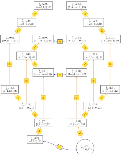
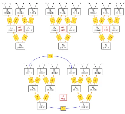
Example 2.11. Consider the partition λ = 21, the graph G21 in Fig. 1 is obtained from the 4-tuple

2

3 1 ,(1,−1,0),(0,0,0),1

by applying the rules of Definition 2.9. In Fig. 1, the steps are drawn in orange, the jumps in blue and the falls have been omitted.

For a reverse standard tableauτ of shape λ, a partition of N, let

inv(τ) = #{(i, j) : 1≤i < j≤N,rw(i, τ)>rw(j, τ)},

where rw(i, τ) is the row of τ containing i(also we denote the column containing iby cl(i, τ)). Then a correct jump fromτ toτ′_{implies inv(τ}′_{) = inv(τ)+1 (the entriesσ[i] andσ[i+1] =σ[i]+1} are interchanged inτ to produce τ′). Thus the number of correct jumps in a path from the root to (τ, ζ, v, σ) equals inv(τ)−inv(τλ).

So we consider the number of steps in a path from 0N _tov;1 _{recall that one step links vtov}′ where either v[i]< v[i+ 1] and v′ =vsi orv′=vΨ.

For x ∈ Z (or R) let ǫ(x) := 1₂(|x|+|x+ 1| −1), then ǫ(x) = x for x ≥ 0, ǫ(x) = 0 for

−1≤x≤0, andǫ(x) =−x−1 forx≤ −1.

There is a symmetry relation: ǫ(x) =ǫ(−x−1).

Definition 2.12. For v∈NN let|v|:=

N

P

i=1

v[i] and set

S(v) := X 1≤i<j≤N

ǫ(v[i]−v[j]).

The above formula can be written as

S(v) = 1 2

X

1≤i<j≤N

(|v[i]−v[j]|+|v[i]−v[j] + 1|)−N(N−1)

4 .

2

It remains to show that S(vΨ) = S(v) (because|vΨ|=|v|+ 1). Note (vΨ)[N] =v[1] + 1. Then

S(v)−S(vΨ) =

N

X

j=2

ǫ(v[1]−v[j])− N

X

i=2

ǫ(v[i]−v[1]−1)

=

N

X

j=2

ǫ(v[1]−v[j])−ǫ(v[j]−v[1]−1) = 0.

This completes the proof.

As a straightforward consequences, Proposition2.13 implies

Corollary 2.14. All the paths joining two given vertices in Gλ have the same length.

This suggests that some properties could be shown by induction on the common length of all the all the paths joining two given vertices.

For a given 4-tuple (τ, ζ, v, σ) the values of ζ and σ are determined by those ofτ and v, as shown by the following proposition.

Proposition 2.15. If (τ, ζ, v, σ) is a vertex inGλ, then σ =σv and ζ[i] =viα+CTτ[σ[i]]. We

will set ζv,τ :=ζ.

Proof . We prove the result by induction on the length k of a path (a1, . . . , ak) (from

Corol-lary2.14 all the paths have the same length) from the root to (τ, ζ, v, σ) and set

(τ′, ζ′, v′, σ′) = τλ,CTτλ,0

N_{,[1, . . . , N]a}

1· · ·ak−1.

Suppose that ak= Ψ is the affine operation. More precisely,τ =τ′,ζ =ζ′Ψα,v=v′Ψ andσ =

σ′[2, . . . , N,1]. Using the induction hypothesis one hasσ′ =σv′ and ζ′[i] =v′[i]α+ CT_τ[σ_v′[i]].

Hence, Proposition 2.4givesσ=σv′_Ψ=σ_v. Suppose thati < N then

ζ[i] =ζ′[i+ 1] =v′[i+ 1]α+ CTτ[σv′[i+ 1]] =v[i]α+ CT_τ[σ_v[i]].

If i=N then again

ζ[i] =ζ′[1] +a= (v′[1] + 1)α+ CTτ[σv′[1]] =v[N]α+ CT_τ[σ_v[N]].

Suppose now thatakis not an affine operation. Using the induction hypothesis one hasσ′ =σv′

and ζ′[j] =v′[j]α+ CTτ[σv′[j]] for eachj. Ifa_k=s_i is a step thenτ =τ′,ζ =ζ′s_i,v=v′s_i and σ =σ′_s

i. Hence, Proposition 2.3 gives σ =σv′_s

i =σv. If j 6=i, i+ 1 then one has ζ[j] = ζ

′_[j],

v[j] =v′[j] andσ[j] =σ′[j], henceζ[j] =v[j]α+ CTτ[σv[j]]. Ifj=ithen one hasζ[i] =ζ′[i+ 1],

v[i] =v′[i+ 1] and σ[i] =σ′[i+ 1], and again the result is straightforward. And similarly when

j=i+ 1 one finds the correct value forζ[i+ 1].

Suppose now that ak =si is a jump. That is τ =τ′(σ[i],σ[i+1]),ζ =ζ′si, v =v′ and σ =σ′.

Straightforwardly,σ =σv′ =σ_v and if j6=i, i+ 1 then

ζ[j] =ζ′[j] =v′[j]α+ CTτ′[σ_v′[j]] =v[j]α+ CT_τ[σ_v[j]].

Suppose that j=i, sinceak is a jumpv′[i] =v′[i+ 1] and

ζ[i] =ζ′[i+ 1] =v′[i+ 1]α+ CTτ′[σ_v′[i+ 1]] =v[i]α+ CT_τ[σ_v[i]].

Example 2.16. Consider the RST τ = 3 7 4 1 8 6 5 2

and the vector v = [6,2,4,2,2,3,1,4].

One has σv = [1,5,2,6,7,4,8,3] and CTτ = [1,3,−2,0,2,1,−1,0] and then

ζv,τ = [6α+ 1,2α+ 2,4α+ 3,2α+ 1,2α−1,3α, α,4α−2].

Hence, the 4-tuple





3 7 4 1 8 6 5 2

,[6α+ 1,2α+ 2,4α+ 3,2α+ 1,2α−1,3α, α,4α−2],[6,2,4,2,2,3,1,4],[1,5,2,6,7,4,8,3]





labels a vertex of G431.

As a consequence,

Corollary 2.17. Let (τ, v) be a pair constituted with a RST τ of shape λ (a partition of N) and a vector v∈ NN. Then there exists a unique vertex in Gλ labeled by a 4-tuple of the form

(τ, ζ, v, σ). We will denoteVτ,ζ,v,σ := (τ, v).

We point out that all the information can be retrieved from the spectral vector ζ – the coefficients of α give v, the rank function of v givesσ, and the constants in the spectral vector give the content vector which does uniquely determine the RSTτ.

Definition 2.18. We define the subgraphGτ as the graph obtained fromGλ by erasing all the

vertices labeled by RST other thanτ and the associated arrows. Such a graph is connected.

Note that the graph Gλ is the union of the graphs Gτ connected by jumps. Furthermore,

ifGτ and Gτ′ are connected by a succession of jumps then there is no step from G_τ′ toG_τ.

Example 2.19. In Fig. 1, the graph G21 is constituted with the two graphs G1

32 and G 2 31 connected by jumps (in blue).

3

Vector-valued polynomials

3.1 About the Young seminormal representation of the symmetric group

We consider the spaceVλ spanned by reverse tableaux of shapeλand the (Young) action of the

symmetric group as defined by Murphy2 in [17] by

τ si=

  

bτ[i]τ ifbτ[i]2 = 1,

bτ[i]τ +τ(i,i+1) if 0< bτ[i]≤ 1₂,

bτ[i]τ + (1−bτ[i]2)τ(i,i+1) otherwise,

(3.1)

where bτ[i] := _CTτ[i]−1_CTτ[i+1]. Note that when |bτ[i]|<1, τ(i,i+1) is always a reverse standard

tableau when τ is a reverse standard tableau.

Murphy showed [17] that the RST are the simultaneous eigenfunctions of the Jucys–Murphy elements:

ωi = N

X

j=i+1 sij,

where sij denotes the transposition exchangingiand j. More precisely:

2_{The Young seminormal representation was defined in Young’s last papers but himself apparently}

Proposition 3.1.

τ ωi = CTτ[i]τ.

As usual, a polynomial representation for the Murphy action on the RST can be computed through the Yang–Baxter graph. We start fromτλ and we construct the associated polynomial

in the variablest1, . . . , tN:

Pτλ =

Y

i

Y

k>l

(i,k),(i,l)∈λ

(t_τλ[i,k]−t_τλ[i,l]),

whereτ[i, j] denotes the integer belonging at the columniand the rowjinτ. Such a polynomial is a simultaneous eigenfunction of the Jucys–Murphy idempotents:

Pτλωi= CTτλ[i]Pτλ.

Suppose that Pτ is the polynomial associated to τ. Suppose also that 0 < bτ[i] < 1. Hence,

the polynomial P_τ(i,i+1) is obtained from the polynomialPτ by acting with si−bτ[i] (with the

standard action of the transpositionsi on the variablestj).

Example 3.2.

P21 43 =P

31 42 s2−

1 2

= (t3−t4)(t1−t2) s2− 1₂

=t1t2− 1₂t4t1− 1₂t3t2+t4t3− 1₂t4t2−1₂t3t1

Let us remark that in [13], Lascoux simplified the Young construction by having recourse to the covariant algebra (of SN) C[x1, . . . , xN]/Sym+ where Sym+ is the ideal generated by symmetric functions without constant terms. Note that the covariant algebra is isomorphic to the regular representation C[SN]. In the aim to adapt his construction to our notations, we

replace each polynomial with its dominant monomial represented by the vectors of its exponents. The vector associated to the root of the graph is the vector exponent of the leading monomial in the product of the Vandermonde determinants associated to each column and is obtained by putting the number of the row minus 1 in the corresponding entry.

Example 3.3. The vector associated to 452

631 is [010210].

In fact, the covariant algebra being isomorphic to the regular representation of SN, the

computation of the polynomials is completely encoded by the action of the symmetric group on the leading monomials, as shown in the following example. Observe that we do not replace the representation by the orbit of the leading monomial (since the space generated by the orbit is in general bigger), but we consider the projection which completely determines the elements.

Example 3.4. Consider the RST of shape 221, one has

3 41 52 2 41 53 1

42 53

2 31 54 1

32 54

[10210] [12010]

[21010] [12100]

[21100]

s2

−

1 3 s

1₋ 1

2 s3−

1 2 s3−

1

2 s1− ₁

2

s2

s

1 s3

For instance, one has

P1 42 53

=t2₁t4t2+₂1t4t22t3+1₂t22t5t1−1₂t22t5t3+1₂t4t23t1+1₂t42t1t3+t21t5t3−t21t5t2+1₂t25t4t3

+ 1₂t5t24t2+ 1₂t25t1t2− 1₂t4t22t1− 1₂t25t4t2+1₂t23t5t2−1₂t24t1t2−t21t4t3−1₂t23t5t1

− 1₂t5t24t3− 1₂t4t23t2− 1₂t25t1t3,

whose leading monomial is t2 1t2t4.

From the construction, the leading monomial of Pτ is the product of all the trw(_i i,τ)−1. For

example, the leading monomial in P51 732 9864

ist2

1t2t3t25t7.

3.2 Def inition and dominance properties of vector-valued polynomials

Consider the space

MN = spanC

xv₁[1]· · ·xv_N[N]⊗τ : v∈NN, τ ∈Tabλ, λ⊢N ,

where Tab(N) denotes the set of the reverse standard tableaux on{1, . . . , N}. This space splits into a direct sumMN =Lλ⊢NMλ, where

Mλ = spanC

xv₁[1]· · ·xv_N[N]⊗τ|v∈NN, τ ∈Tabλ .

The algebra C[SN]⊗C[SN] acts on these spaces by commuting the vector of the powers on

the variables on the left component and the action on the tableaux defined by Murphy (equa-tion (3.1)) on the right component.

Example 3.5.

x3₁x1₂⊗ 2

3 1 (s2⊗s1) = 1 2x

3 1x13⊗

2

3 1 +x 3 1x13⊗

1 3 2 .

For simplicity we will denote xv _{= x}v[1]

1 · · ·x

v[N]

N and xv,τ := xv ⊗τ σv. By abuse of

lan-guagexv,τ _{will be referred to as a polynomial. Note that the spaceM}

λ is spanned by the set of

polynomials

Mλ :=xv,τ :v∈NN, τ ∈Tabλ ,

which can be naturally endowed with the order✁ defined by

xv,ττ ✁xv′,τ′ iffv✁v′,

withv✁v′ _{means thatv}+_≺v′+_orv+_=v′+_andv≺v′_{, where≺denotes the classical dominance} order on vectors:

vv′ iff ∀i, v[1] +· · ·+v[i]≤v′[1] +· · ·+v′[i].

Example 3.6.

1. x031,

2

3 1 _✁x310, 1

3 2 _{since 031≺310.}

2. x220,

2

3 1 _✁x301, 1

3 2 _{since 220≺310.}

3. The polynomials x031,

2

3 1 _{and x}031, 1

The partial order✂will provide us a relevant dominance notion.

Definition 3.7. The monomialxv,τ is theleading monomialof a polynomial P if and only ifP

can be written as

P =αvxv,τ+

X

xv′,τ′✁xv,τ

αv′_,τ′xv ′_,τ′

with αv 6= 0.

As in [9], we define Ψ := (θ⊗θ)xN, with θ = s1s2· · ·sN−1. The following proposition describes the transformation properties of leading monomials with respect to the si and Ψ.

Proposition 3.8. Suppose that xv,τ is the leading monomial in P then

1. If v[i]< v[i+ 1] thenxvsi,τ _{is the leading monomial inP(s}

i⊗si). Its leading monomial is

x˜v⊗(τ.sij), where xv˜ is the dominant term in ∂ijx˜v.

2. xvΨ,τ is the leading monomial in PΨ.

3.3 Dunkl and Cherednik–Dunkl operators for vector-valued polynomials

We define the Dunkl operators

Di:=

∂ ∂xi

⊗1 + 1

α

X

i6=j

∂ij⊗sij,

where sij denotes the transposition which exchangesiand j and

∂ij = (1−sij)

1

xi−xj

is the divided difference.

This definition is the same as in [4], but our operators act on their left. One has

Lemma 3.9. If Di denotes the Dunkl operator, one has

(si⊗si)Di =Di+1(si⊗si).

Proof . Straightforward from the definition of Di and the equalities

sisij =si+1,jsi, si∂ij =∂i+1jsi and si

∂ ∂xi

= ∂

∂xi+1

si.

The Cherednik–Dunkl operators are pairwise commuting operators defined by [4]

Ui:=xiDi−

1

α

i−1 X

j=1

si,j⊗si,j.

We do not repeat the proof of the commutation [Ui,Uj] = 0 which can be found in [4]. But, as we

will see in the next section, this property is not used to prove the existence of the vector-valued Jack polynomials.

One has

Lemma 3.10.

2. (si⊗si)Uj =Uj(si⊗si), j6=i, i+ 1.

3. (si⊗si)Ui+1 =Ui(si⊗si)−_α1.

Proof . The three identities are of the same type. We prove only the first one which follows from the equalities

(si⊗si)Ui = (si⊗si)xiDi−

1

α

i−1 X

j=1

si,j⊗si,j

= 

xi+1Di+1− 1

α

i−1 X

j=1

si+1,j⊗si+1,j



(si⊗si) =Ui+1(si⊗si) +

1

α.

The affine operator Ψ has the following commutation properties with the Dunkl operators:

Lemma 3.11.

1. Di+1Ψ = ΨDi+ (θ⊗θ)(si,N ⊗si,N), i <1.

2. D1Ψ = ΨDN+ (θ⊗θ) N_P−1

j=1

(sN,j ⊗sN,j)−1

! .

As a consequence, one finds.

Lemma 3.12.

ΨUi =Ui+1Ψ, i=6 N and ΨUN = (U1+ 1) Ψ.

The action on the RST is given by

Lemma 3.13.

(1⊗τ)Ui=

1 + 1

αCTτ[i]

(1⊗τ).

Proof . One has

(1⊗τ)Ui= (1⊗τ)xiDi−

1

α

i−1 X

j=1

(1⊗τ)(si,j⊗si,j) = (1⊗τ)

1 + 1

α1⊗ωi

,

where ωi := N

P

j=i+1

(i j) denotes a Jucys–Murphy element. Since the RST are eigenfunctions of

the Jucys–Murphy elements and the associated eigenvalues are given by the contents, the lemma

follows.

For convenience, define ˜ξi :=αUi−α. From the preceding lemmas, one obtains

Proposition 3.14.

(si⊗si) ˜ξi= ˜ξi+1(si⊗si) + 1,

(si⊗si) ˜ξi+1= ˜ξi(si⊗si)−1,

(si⊗si) ˜ξj = ˜ξj(si⊗si), j6=i, i+ 1,

Ψ ˜ξi = ˜ξi+1Ψ, i6=N,

4

Nonsymmetric vector-valued Jack polynomials

In this section we recover the construction, due to one of the authors [4], of a basis of vector-valued polynomials Jv,τ. This construction belongs to a large family of vector-valued Jack

polynomials associated to the complex reflection groups G(r,1, n) defined by Griffeth [8]. We will denote by ζv,τ their associated spectral vectors. We will see also that many properties of

this basis can be deduced from the Yang–Baxter structure.

4.1 Yang–Baxter construction associated to Gλ

Let λ be a partition and Gλ be the associated graph. We construct the set of polynomials

(JP)_{Ppath in Gλ} using the following recursive rules:

1. J[] := (1⊗τλ).

2. If P= [a1, . . . , ak−1, si] then

JP:=J[a1,...,ak−1]

si⊗si+

1

ζ[i+ 1]−ζ[i]

,

where the vector ζ is defined by

(τλ,CTτλ,0

N_{,[1,2, . . . , N])a}

1. . . ak−1 = (τ, ζ, v, σ).

3. If P= [a1, . . . , ak−1,Ψ] then

JP=J[a1,...,ak−1]Ψ.

One has the following theorem.

Theorem 4.1. Let P = [a0, . . . , ak] be a path in Gλ from the root to (τ, ζ, v, σ). The

polyno-mial JP is a simultaneous eigenfunctions of the operators ξ˜i whose leading monomial is xv,τ.

Furthermore, the eigenvalues of ξ˜i associated to JP are equal to ζ[i].

Consequently JP does not depend on the path, but only on the end point (τ, ζ, v, σ), and will

be denoted by Jv,τ. The family (Jv,τ)v,τ forms a basis of Mλ of simultaneous eigenfunctions of

the Cherednik operators.

Furthermore, ifP leads to ∅ thenJP= 0.

Proof . We will prove the result by induction on the length k. If k= 0 then the result follows from Proposition 3.13. Suppose now that k >0 and let

(τ′, ζ′, v′, σv′) = τ_λ,CT_τ λ,0

N_{,[1, . . . , N]a}

1· · ·ak−1.

By induction, J_[a1,...,ak−1] is a simultaneous eigenfunctions of the operators ˜ξi such that the associated vector of eigenvalues is given by

J_[a1,...,ak−1]ξ˜i=ζ ′_[i]J

[a1,...,ak−1]

and the leading monomial is xv′_,τ′

.

If ak = Ψ is an affine arrow, then τ = τ′, ζ = ζ′.Ψα, v = v′Ψ, σv = σv′[2, . . . , N,1] and JP =J[a1,...,ak−1]Ψ. If i6=N

JPξ˜i =J[a1,...,ak−1]Ψ ˜ξi =J[a1,...,ak−1]ξ˜i+1Ψ =ζ

′_{[i+ 1]J}

Ifi=N then,

JPξ˜N =J[a1,...,ak−1]Ψ ˜ξN =J[a1,...,ak−1]˜(ξ1+α)Ψ = (ζ

′_{[1] +α)J}

P =ζ[N]JP.

The leading monomial is a consequence of Proposition 3.8.

=xv⊗(τ′sσ_v′[i]σv′) +

1

ζ′_{[i+ 1]−ζ}′_[i]x

v′

⊗(τ′σv′)

=xv⊗(τ σv) +

b′_τ[σv′[i]] + 1 ζ′_{[i+ 1]−ζ}′_[i]

xv′⊗(τ′σv′)

=xv,τ +

b′_τ[σv′[i]] +

1

ζ′_{[i+ 1]−ζ}′_[i]

xv′,τ′.

But ζ′[i] = CTτ′[σ_v′[i]] and ζ′[i+ 1] = CT_τ′[σ_v′[i+ 1]] = CT_τ′[σ_v′[i] + 1], hence b_τ′[σ_v′[i]] =

−_ζ′_[i+1]1_−ζ′_[i]. And the leading monomial isQ=xv,τ as expected.

This proves the first part of the theorem and that the family (Jv,τ)v,τ forms a basis ofMλ of

simultaneous eigenfunctions of the Cherednik operators. Finally, ifak=si is a fall, Q is proportional toxv

′

⊗(τ′_σ

v′) and thenJ_P is proportional to J[a1,...,ak−1]. But clearly, the two polynomials are eigenfunction of the Cherednik operators with different eigenvalues from the cases j=iand j=i+ 1. This proves that JP= 0.

As a consequence, we will consider the family of polynomials (Jv,τ)v,τ indexed by pairs (v, τ)

where v∈NN is a weight and τ is a tableau.

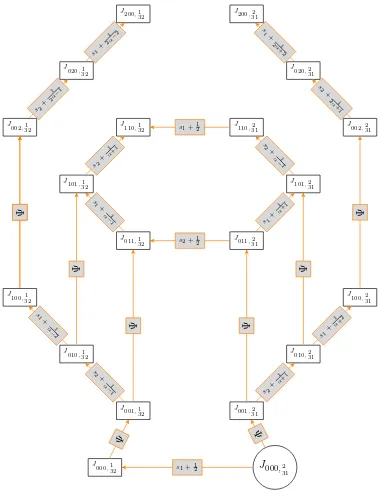
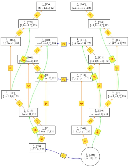
Example 4.2. For λ = 21, the first polynomials Jv,τ are displayed in Fig. 2. The spectral

vectors can be read on Fig. 1.

Note that if [a1, . . . , ak−1] leads to a vertex other than ∅ and [a1, . . . , ak−1, si] leads to ∅,

the last part of Theorem 4.1 implies that J[a1,...,ak−1] is symmetric or antisymmetric under the action of si⊗si.

The recursive rules of this section first appeared in [8]. The Lemma 5.3 and the Yang–Baxter graph constitute essentially what Griffeth called calibration graphin that paper.

4.2 Partial Yang–Baxter-type construction associated to Gτ

To compute an expression for a polynomial Jv,τ it suffices to find the good path in the

sub-graph Gτ as shown by the following examples.

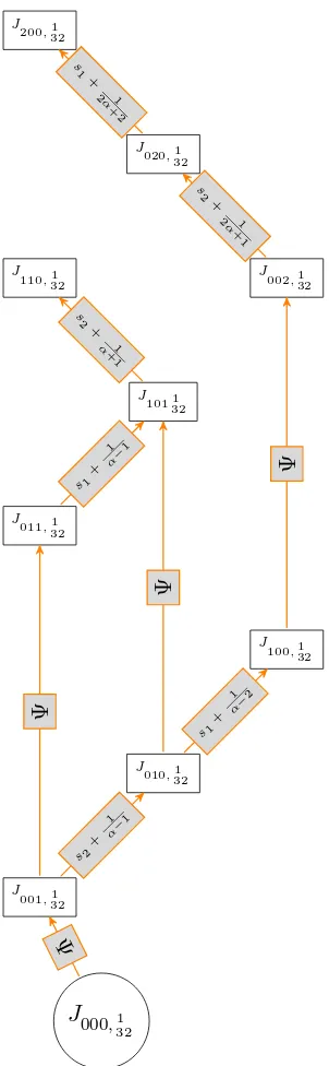
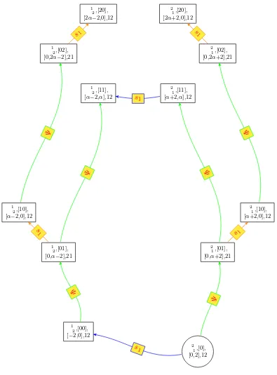
Example 4.3. Considerτ = 1

3 2 , Fig. 3explains how to obtains the values ofJv,₃₂1 from the

graph G1 32.

Example 4.4. For the trivial representation (i.e.,λhas a single part), note that the Cherednik operators (in [14]) have the same eigenspaces as the Cherednik–Dunkl operators Ui (in [4]). In

the notations of [14],ξi reads

ξi =αxi

∂ ∂xi

+

N

X

j=1

j6=i

πij + (1−i),

where

πij =

xi∂ij ifj < i,

xj∂ij ifi < j,

where∂ij denotes the divided difference on the variablesxiandxj. Noting thatxi∂ij =∂ijxi−1,

xj∂ij =∂ijxi−(ij) and xi_∂x∂_i = _∂x∂_ixi−1, one finds

J_000,2

Example 4.5. Consider sign representation associated to the partition [1N_{]. The set Tab}

[1N_]

contains a unique element τ = 1

.. .

N

. Hence, we can omit τ when we write the polynomials

of M_[1N_]. One can see that the corresponding Jack polynomials are equal to the standard ones

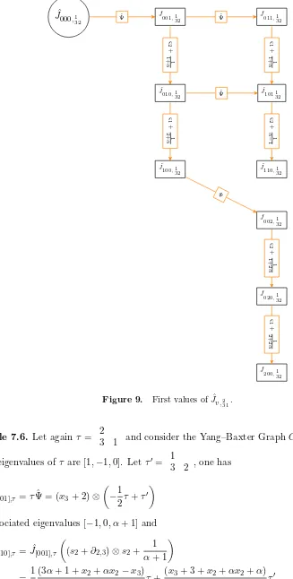
J_000,1 32

J

001,₃₂1

J

010,₃₂1

J

100,₃₂1

s2+ 1

α−

1

s1+ 1

α−

2

Ψ

J

011,₃₂1

J

1011₃₂

J

002,₃₂1

Ψ

Ψ

Ψ

s1+ 1

α−

1 J

110,₃₂1

s 2₊

1

α

+ 1

J

020,₃₂1

J

200,₃₂1

s 2₊

1 2α

+ 1 s

1₊

1 2α

+ 2

Figure 3. First values of the polynomialsJ_v,1 32.

Hence, the Cherednik–Dunkl operatorUi =xiDi−_α1 i_P−1

j=1

sij⊗sij acts onM[1N_]as the operatorU_i

acts on M_[N] but for the parameter −α.

Example 4.6. Let us explain the method on a bigger example: J_[0,0,2,1,1,0],τ, for τ :=

4 3 6 5 2 1. First, we obtain the vector [0,0,2,1,1,0] from [0,0,0,0,0,0] by the following sequence of opera-tions:

[0,0,0,0,0,0] →Ψ [0,0,0,0,0,1] →s5 [0,0,0,0,1,0] →s4 [0,0,0,1,0,0] →s3 [0,0,1,0,0,0]

s2

s5

→[0,0,0,2,1,0] →Ψ [0,0,2,1,0,1] →s5 [0,0,2,1,1,0].

Replace Ψ by Ψα _{in the list of the operations, the associated sequence is}

ζ_[0,0,0,0,0,0]= [3,2,0,−1,1,0] Ψα

→ ζ_[0,0,0,0,0,1]= [2,0,−1,1,0, α+ 3]

s5

→ ζ_[0,0,0,0,1,0]= [2,0,−1,1, α+ 3,0]

s4

→ ζ_[0,0,0,1,0,0]= [2,0,−1, α+ 3,1,0]

s3

→ ζ[0,0,1,0,0,0]= [2,0, α+ 3,−1,1,0]

s2

→ ζ[0,1,0,0,0,0]= [2, α+ 3,0,−1,1,0]

s1

→ ζ_[1,0,0,0,0,0]= [α+ 3,2,0,−1,1,0] Ψα

→ ζ_[0,0,0,0,0,2]= [2,0,−1,1,0,2α+ 3]

s5

→ ζ_{[0,0,0,0,2,0]}= [2,0,−1,1,2α+ 3,0] Ψ→α ζ_{[0,0,0,2,0,1]}= [0,−1,1,2α+ 3,0, α+ 2]

s5

→ ζ_[0,0,0,2,1,0]= [0,−1,1,2α+ 3, α+ 2,0] Ψα

→ ζ_[0,0,2,1,0,1] = [−1,1,2α+ 3, α+ 2,0, α]

s5

→ ζ[0,0,2,1,1,0]= [−1,1,2α+ 3, α+ 2, α,0].

Now, to obtain the vector-valued Jack polynomial, it suffices to start from 1⊗ 4 3

6 5 2 1 and act successively with the affine operator Ψ (when reading Ψα_{) and withs}

i⊗si+_ζ[i+1]1_−ζ[i]

(when reading si).

In conclusion, the computation of vector-valued Jack for a given RST is completely indepen-dent of the computations of the vector-valued Jack indexed by the other RST with the same shape.

4.3 Normalization

The space Vλ spanned by the RST τ of the same shape λ is naturally endowed (up to a

mul-tiplicative constant) by SN-invariant scalar product h,i0 with respect to which the RST are pairwise orthogonal. As in [4], we set

||τ||2 = Y 1≤i<j≤N

CTτ[i]<CTτ[j]−1

(CTτ[i]−CTτ[j]−1)(CTτ[i]−CTτ[j] + 1)

(CTτ[i]−CTτ[j])2

.

As in [4], we consider the contravariant form h , i on the space Mλ which is the symmetric

SN-invariant form extending h,i0 and such that the Dunkl operator Di is the adjoint to the

multiplication by xi (see appendix in [4] for more details).

The operator xiDi is self adjoint and the adjoint of σ ∈ SN is σ−1. Since sij =s−_ij1 is self

adjoint,Ui is self-adjoint for the form h , i and the polynomialsJv,τ are pairwise orthogonal.

Let us compute their squared norms||Jv,τ||2 (the bilinear form is nonsingular for generic α

and positive definite forαin some subset ofR[6]). The method is essentially the same as in [4] and we show that the result can be read in the Yang–Baxter graph. More precisely, one has

Proposition 4.7.

1. ||J₍v,τ)si||

2₌ (ζv,τ[i+ 1]−ζv,τ[i]−1)(ζv,τ[i+ 1]−ζv,τ[i] + 1)

(ζv,τ[i+ 1]−ζv,τ[i])2

||Jv,τ||2.

2. ||J(v,τ)Ψ||2 =

1

αζv,τ[1] + 1

||Jv,τ||2.

Proof . 1. Since

J₍v,τ)si =Jv,τ

si⊗si+

1

ζv,τ[i+ 1]−ζv,τ[i]

J_000,1 32

J

001,1₃₂

J

010,₃₂1

J

100,1₃₂

×α(α+2)

(α+1)2

×(α+1)(α+3)

(α+2)2

×_α1+ 1 J011,1₃₂

J

101₃₂1

J

002,1₃₂

×−_α1 + 1

×−_α1+ 1

×_α1+ 2

×α(α+2)

(α+1)2

J

110,1₃₂

×(α−2)α

(α−1)2

J

020,1₃₂

J

200,1₃₂

×2α(2α+2)

(2α+1)2

×(2α+1)(2α+3)

(2α+2)2

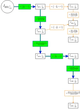
Figure 4. Computation of||J020,1₃₂||

2

using the graph G1 32.

one obtains

||Jv,τ(si⊗si)||2=||J(v,τ)si||

2₊ 1

(ζv,τ[i+ 1]−ζv,τ[i])2

||Jv,τ||2.

But ||Jv,τ(si⊗si)||2 =||Jv,τ||2, which gives the result.

2. One has

||J₍v,τ)Ψ||2 =||Jv,τ(θ⊗θ)xN||2=hJv,τ(θ⊗θ), Jv,τ(θ⊗θ)xNDNi

=hJv,τ(θ⊗θ), Jv,τx1D1(θ⊗θ)i=hJv,τ, Jv,τx1D1i;

recall thatθ=s1s2· · ·sN−1. Since U1=x1D1, one obtains the results.

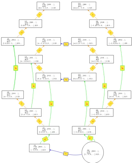
Example 4.8. Let againτ = 2

3 1 , we compute the normalization following the Yang–Baxter graph (see Fig. 4).

For instance:

||J[020],τ||2=||τ||2

1 + 1

α

α(α+ 2) (α+ 1)2

(α+ 1)(α+ 3)

(α+ 2)2 2 + 1

α

2α(2α+ 2) (2α+ 1)2

5

Symmetrization and antisymmetrization

In [2], Baker and Forrester investigated the coefficients and the norm of the symmetric Jack polynomials by symmetrizing the nonsymmetric Jack polynomials. The symmetrization method was used in [5] for the polynomials associated with the complex groups G(r, p, N). In this section, we generalize their results and obtain symmetric and antisymmetric vector-valued Jack polynomials.

5.1 Non-af f ine connectivity

Let us denote byHλ the graph obtained fromGλ by removing the affine edges, all the falls and

the vertex ∅. The purpose of this section is to investigate the connected components of Hλ.

Recall that v+ _{is the unique decreasing partition obtained by permuting the entries ofv.}

Definition 5.1. Letv∈NN andτ ∈Tabλ (λpartition). We define the fillingT(τ, v) obtained

by replacing iby v+_{[i] inτ for each i.}

Proposition 5.2. Two 4-tuples (τ, ζ, v, σ) and (τ′, ζ′, v′, σ′) are in the same connected compo-nent of Hλ if and only if T(τ, v) =T(τ′, v′).

Proof . Remark first that the steps and correct jumps preserve T(τ, v). Indeed steps leave invariant the pairs (τ, v+) whilst the correct jumps act on the RST byτ sσv[i]wherev[i] =v[i+1]

(or equivalently byτ sj wherev+[j] =v+[j+ 1]. Hence, we show that if (τ, ζ, v, σ) is connected

to (τ′, ζ′, v′, σ′) thenT(τ, v) =T(τ′, v′).

Let us prove the converse. Suppose that T(τ, v) = T(τ′, v′). Since (τ, ζ, v, σ) (resp. (τ′, ζ′,

v′_{, σ}′_{)) is connected to (τ, ζ, v}+_{,Id) (resp. (τ}′_{, ζ}′_{, v}′+_{,Id)) by steps, it suffices to prove the result} forT(τ, µ) =T(τ′, µ) whenµis a (decreasing) partition. Letρ∈SN such thatτρ(the tableauτ

where the entries have been permuted by ρ) equals τλ. By construction T(τ, µ) = T(τλ, µρ−1)

and then it suffices to show the result forT(τλ, µρ−1) =T(τ′ρ, µρ−1). Again the connectivity by

steps implies that it suffices to prove the result forT(τλ, µ) =T(τ′, µ) whenµis a partition. We

will show that if T(τλ, µ) =T(τ, µ) then there exists a series of correct jumps from (τ, ζ′, µ,Id)

to (τλ, ζ, µ,Id) when µ is a partition. We prove the result by induction on the length of the

shortest permutation ω such thatτ ω =τλ for the weak order. The base point of the induction

is straightforward. Now, choose i such that ω[i] > ω[i+ 1] and i and i+ 1 are neither in the same row nor in the same column in τ then ω = siω′ where ℓ(ω′) < ℓ(ω). Since T(τ, µ) =

T(τ′, µ), this means thatµ[i] =µ[i+ 1] and hence, there is a correct jump from (τ, ζ′, µ,Id) to (τ(i,i+1)_{, ζ}′_s

i, µ,Id). By the induction hypothesis, this shows the result.

This shows that the connected components of Hλ are indexed by the T(τ, µ) where µ is

a partition.

Definition 5.3. We will denote byHT the connected component associated toT inHλ. The

componentHT will be said to be 1-compatibleifT is a column-strict tableau. The componentHT

will be said to be (−1)-compatibleifT is a row-strict tableau.

Example 5.4. Let µ= [2,1,1,0,0] andλ= [3,2]. There are four connected components with vertices labeled by permutations of µinHλ (see Fig.5). The possible values of T(τ, µ) are

12 001,

02 011,

01

012 and

11 002,

squared in red in Fig. 5. The 1-compatible components are H12

001 and H 11

002 while there is only one (−1)-compatible componentH01

012. The componentH 02

011 is neither 1-compatible nor (− 1)-compatible.

The componentH12

001 contains vertices ofG 31

542 and G 21

41

Figure 5. Some connected components ofH32.

We we use the following result in the sequel, its proof is easy and left to the reader.

Proposition 5.5. Let (τ, ζ, v, σ) be a vertex of HT such that(τ, ζ, v, σ)si =∅. One has

1. If HT is1-compatible then σ[i]and σ[i+ 1](=σ[i] + 1) are in the same row in τ.

2. If HT is(−1)-compatible then σ[i] andσ[i+ 1](=σ[i] + 1) are in the same column inτ.

The following definition is used to find a RST corresponding to a filling of a shape.

Definition 5.6. Let T be a filling of shape λ, the standardization std(T) of T is the reverse standard tableau with shape λobtained by the following process:

1. Denote by |T|i the number of occurrences of i inT

2. Read the tableau T from the left to the right and the bottom to the top and replace successively each occurrence ofiby the numbersN− |T|0− · · · − |T|i−1,N − |T|0− · · · −

|T|i−1−1, . . . ,N − |T|0− · · · − |T|i.

Alternatively, one has

std(T) [i, j] := #{(k, l) :T[k, l]> T[i, j]}+ #{(k, l) :l > j, T[k, l] =T[i, j]}

+ #{(k, j) :k≥i, T [k, j] =T[i, j]}.

We will denote by λT the unique partition obtained by sorting in the decreasing order all the

Example 5.7. Pictorially, reading 01₀₀₂ one obtains

0 0 2 0 1

0 0 . 0 .

. . . . 1

. . 2 . .

Renumbering in increasing order from the bottom to the top and the right to the left, one reads

0 0 2 0 1

5 4 . 3 .

. . . . 2

. . 1 . .

Hence, we have std ₀₀₂01 = ₅₄₁32 and λ01

002 = [21000].

Note that eachHT has a unique sink (that is a vertex with no outward edge) and this vertex

is labeled by (std(T), ζT, λT,Id) for a certain vectorζT and a unique root.

Example 5.8. Consider the tableau T = 01₀₀. Its standardization is std(T) = 21₄₃ and the graph HT is:

31 42 [0001]

31 42 [0010]

31 42 [0100]

31 42 [1000] 21

43 [0001]

21 43 [0010]

21 43 [0100]

21 43 [1000]

s1 _s1

s2

s3 s2 s1

s3 s2 s1

The sink is denoted by a red disk and the root by a green disk.

5.2 Symmetric and antisymmetric Jack polynomials

For convenience, let us define:

(v, τ)si = (v′, τ′) if (τ, ζ, v, σ)si = (τ′, ζ′, v′, σ′)

and

(v, τ)si =∅ if (τ, ζ, v, σ)si=∅.

Denote also, J∅:= 0.

Let (τ, ζ, v, σ) be a vertex of HT, set bv,τ[i] = _ζv,τ[i+1]1_−ζv,τ[i] and cv,τ[i] = _ζv,τζv,τ_[i[_]−i]−_ζv,τζv,τ_[i+1]+1[i+1] .

Note that

1 +cv,τ[i]bv,τ[i] =cv,τ[i] (5.1)

and

cv,τ[i](1−bv,τ[i]2)−bv,τ[i] = 1. (5.2)

Let HT be a 1-compatible component of Gλ. For each vertex (τ, ζ, v, σ) of HT, we define the

1. Ev,τ = 1 if there is no arrows of the form

(τ′, ζ′, v′, σ′₎ si (τ, ζ, v, σ)

inHT.

2. Ev,τ = ζ

′_[i+1]−ζ′_[i]

ζ′_[i+1]−ζ′_[i]−1Ev′_,τ′ = ζ[i+1]−ζ[i]

ζ[i+1]−ζ[i]+1Ev′,τ′ =cv′,τ′Ev′,τ′ if there is an arrow

(τ′, ζ′, v′, σ′₎ si (τ, ζ, v, σ)

inHT.

The symmetric group acts on the spectral vectorsζ by permuting their components. Hence the value ofEv,τ does not depend on the path used for its computation and theEv,τ are well defined.

Indeed, it suffices to check that the definition is compatible with the commutations sisj =sjsi

with |i−j|>1 and the braid relations sisi+1si =si+1sisi+1.

Let us first prove the compatibility with the commutation relations. Suppose

(τ0, ζ0, v0, σ0)sisj = (τ1, ζ1, v1, σ1)sj = (τ2, ζ2, v2, σ2),

with |i−j|>1 and

(τ0, ζ0, v0, σ0)sjsi= (τ1′, ζ1′, v′1, σ′1)si= (τ2′, ζ2′, v2′, σ′2).

Note that τ₂′ =τ2, ζ2′ =ζ2, v2′ =v2 and σ′2 =σ2. But, since the symmetric group acts on ζ by permuting its components, one has

ζ2[j+ 1] =ζ1′[j+ 1], ζ2[j] =ζ1′[j], ζ1[j+ 1] =ζ2′[j+ 1] and ζ1[j] =ζ2′[j].

Hence,

ζ2[j+ 1]−ζ2[j] ζ2[j+ 1]−ζ2[j] + 1

. ζ1[i+ 1]−ζ1[i] ζ1[i+ 1]−ζ1[i] + 1

= ζ1[i+ 1]−ζ1[i]

ζ1[i+ 1]−ζ1[i] + 1

. ζ2[j+ 1]−ζ2[j] ζ2[j+ 1]−ζ2[j] + 1

= ζ

′

1[i+ 1]−ζ1′[i] ζ′

1[i+ 1]−ζ1′[i] + 1 . ζ

′

2[j+ 1]−ζ2′[j] ζ′

2[j+ 1]−ζ2′[j] + 1 ,

and the definition ofEv,τ is compatible with the commutations.

Now, let us show that the definition is compatible with the braid relations and set

(τ0, ζ0, v0, σ0)sisi+1si = (τ1, ζ1, v1, σ1)si+1si = (τ2, ζ2, v2, σ2)si = (τ3, ζ3, v3, σ3),

and

(τ0, ζ0, v0, σ0)si+1sisi+1 = (τ1′, ζ1′, v′1, σ1′)sisi+1 = (τ2′, ζ2′, v′2, σ2′)si+1= (τ3′, ζ3′, v3′, σ′3).

Note that τ′

3 = τ3, ζ3′ = ζ3, v3′ = v3 and σ3′ = σ3. Since the symmetric group acts on ζ by permuting its components, one has

ζ3[i+ 1] =ζ1′[i+ 1], ζ3[i] =ζ1′[i+ 1], ζ2[i+ 2] =ζ2′[i+ 1], ζ2[i+ 1] =ζ2′[i],

Hence,

ζ3[i+ 1]−ζ3[i] ζ3[i+ 1]−ζ3[i] + 1

. ζ2[i+ 2]−ζ2[i+ 1] ζ2[i+ 2]−ζ2[i+ 1] + 1

. ζ1[i+ 1]−ζ1[i] ζ1[i+ 1]−ζ1[i] + 1

= ζ1[i+ 1]−ζ1[i]

ζ1[i+ 1]−ζ1[i] + 1

. ζ2[i+ 2]−ζ2[i+ 1] ζ2[i+ 2]−ζ2[i+ 1] + 1

. ζ3[i+ 1]−ζ3[i] ζ3[i+ 1]−ζ3[i] + 1

= ζ

′

3[i+ 2]−ζ3′[i+ 1] ζ₃′[i+ 2]−ζ₃′[i+ 1] + 1.

ζ′

2[i+ 1]−ζ2′[i] ζ₂′[i+ 1]−ζ₂′[i] + 1.

ζ′

1[i+ 2]−ζ1′[i+ 1] ζ₁′[i+ 2]−ζ₁′[i+ 1] + 1,

and the definition is compatible with the braid relations. Define the symmetrization operator

S:= X

ω∈SN ω⊗ω.

We will say that a polynomial is symmetric if it is invariant under the action ofsi⊗si for

each i < N.

Theorem 5.9.

1. Let HT be a connected component of Gλ. For each vertex (τ, ζ, v, σ) of HT, the

polyno-mial Jv,τSequals JλT,std(T)Sup to a multiplicative constant.

2. One has JλT,std(T)S6= 0 if and only if HT is 1-compatible.

3. More precisely, when HT is1-compatible, the polynomial

JT =

X

(τ,ζ,v,σ) vertex of HT

Ev,τJv,τ

is symmetric.

Proof . 1. Let us prove the first assertion by induction on the length of a path from (τ, ζ, v, σ) to (std(T), ζT, λT, σ) in HT. Let (τ′, ζ′, v′, σ′) such that

(τ, ζ, v, σ) si (τ′_{, ζ}′_{, v}′_{, σ}′₎

is not a jump in HT (hence,−1< bv,τ[i]<1). It follows that

Jv,τS=

1 1−bv,τ[i]2

Jv′_,τ′(s_i⊗s_i) +b_v,τ[i]J_v′_,τ′S= 1

1−bv,τ[i]2

(1 +bv,τ[i])Jv′_,τ′S.

By induction Jv′_,τ′Sis proportional toJ_λ

T,std(T), which ends the proof.

2. If HT is not 1-compatible, then there existssi such thatJλT,std(T)(si⊗si) =−JλT,std(T).

Hence, since S= (si⊗si)S, one obtainsJλT,std(T)S= 0.

3. Let us prove that, when HT is 1-compatible, JT(si ⊗si) = JT for any i. Fix i and

decompose JT :=J++J0+J− where

J+=X

τ,v

+

Eτ,vJv,τ,

where P+ means that the sum is over the pairs (τ, v) such that there exists an arrow

inHT,

J−=X

τ,v

−

Eτ,vJv,τ

where P− means that the sum is over the pairs (τ, v) such that there exists an arrow

(τ, ζ, v, σ) si (τ′, ζ′, v′, σ′₎

inHT and

J0 = X0

Eτ,vJv,τ,

where P0 means that the sum is over the pairs (τ, v) such that there exists an arrow

(τ, ζ, v, σ) si ∅

inGT (equivalently there is no arrow from (τ, ζ, v, σ) labeled bysi inHT). Suppose that

(τ, ζ, v, σ) si ∅

is a fall in GT, then

Jv,τ(si⊗si) =J(v,τ)si−bv,τ[i]Jv,τ =−bv,τ[i]Jv,τ.

Since, HT is 1-compatible Proposition5.5implies thati andi+ 1 are in the same row. Hence,

bv,τ[i] =−1 and Jv,τ(si⊗si) =Jv,τ. It follows that J0(si⊗si) =J0. Now, let

(τ, ζ, v, σ) si (τ′_{, ζ}′_{, v}′_{, σ}′₎

be an arrow inHT, then

Jv,τ(si⊗si) =Jv′_,τ′ −b_v,τ[i]J_v,τ,

Jv′_,τ′(s_i⊗s_i) =b_v,τ[i]J_v′_,τ′ + (1−b_v,τ[i]2)J_v,τ and E_v′_,τ′ =c_v,τE_v,τ.

Hence, equalities (5.1) and (5.2) imply

(Ev,τJv,τ +Ev′_,τ′J_v′_,τ′)(s_i⊗s_i) =E_v,τ(J_v,τ+c_v,τ[i]J_v′_,τ′)(s_i⊗s_i)

=Ev,τ ((cv,τ[i](1−bv,τ[i]2)−bv,τ[i])Jv,τ+ (1 +cv,τ[i]bv,τ[i])Jv′_,τ′

=Ev,τ(Jv,τ+cv,τ[i]Jv′_,τ′) = (E_v,τJ_v,τ+E_v′_,τ′J_v′_,τ′).

This proves that (J++J−)(si⊗si) = J++J−. Hence, JT(si⊗si) =JT for each iand JT is

symmetric.

Example 5.10. Consider the graph H11 00

21 43 [0011]

21 43 [0101]

21 43 [0110]

21 43 [1001]

21 43 [1010]

21 43 [1100] s2

× α α−1

s₁ ×_α

− 1

α

− 2

s3 ×

α−

1

α−

2

s₁ ×_α

− 1

α

− 2

s3 ×

α−

1

α−

2

The polynomial

J11

00 =J0011, 21 43 +

α

α−1J0101,21₄₃ +

α

α−2J0110,21₄₃ +

α

α−2J1001,21₄₃ +

α(α−1)

(α−2)2J1010,21₄₃

+ α(α−1)

(α−2)(α−3)J1100,21₄₃

is symmetric.

LetHT be a connected component, denote by root(T) the only vertex ofHT without inward

edge and by sink(T) = (std(T), ζT, λT,Id) the only vertex of HT without outward edge.

De-note by #HT the number of vertices of HT. The following proposition allows to compare the

polynomial JT to the symmetrization of Jroot(T).

Proposition 5.11. One has

JT =

#HT

N! Esink(T)Jroot(T)S.

Proof . It suffices to compare the coefficient ofJsink(T) inJT and inJroot(T).S. The coefficient of J_sink(T) inJT equals Esink(T) while the coefficient of Jsink(T) inJroot(T)Sequals #NH!. Indeed

N!

#H is the order of the stabilizer ofλT. The leading monomial ofJsink(T)does not appear in any otherJv,τso its coefficient in the symmetrization ofJroot(T)equals the order of the stabilizer.

LetHT be a (−1)-compatible component ofGλ. For each vertex (τ, ζ, v, σ) ofHT, we define

the coefficientFv,τ by the following induction:

1. Fv,τ = 1 if there is no arrow of the form

(τ′_{, ζ}′_{, v}′_{, σ}′₎ si ₍τ, ζ, v, σ)

inHT.

2. Fv,τ =−_ζ[ζ_i][i₋]−_ζ[ζ_i+1]+1[i+1] Fv′_,τ′ =− ζ

′_{[i+1]−ζ[i]}

ζ′_{[i+1]−ζ[i]+1}Fv′_,τ′ if there is an arrow

(τ′_{, ζ}′_{, v}′_{, σ}′₎ si ₍τ, ζ, v, σ)

inHT.

Again the Fv,τ are well defined since the symmetric group acts on the spectral vectors by

permuting their components. Define also the antisymmetrization operator

A:= X

ω∈SN

(−1)ℓ(ω)(ω⊗ω).

We will say that a polynomial is antisymmetric if it vanishes under the action of 1−si⊗si

for each i < N.

Theorem 5.12.

1. Let HT be a connected component of Gλ. For each vertex (τ, ζ, v, σ) of HT, the

polyno-mial Jv,τA equals JλT,std(T)A up to a multiplicative constant.

3. More precisely, when HT is(−1)-compatible, the polynomial

Example 5.13. Consider the graph H01 01

And, as in the symmetric case, one has:

Proposition 5.14. One has

JT =

#HT

N! Fsink(T)Jroot(T).A.

5.3 Normalization

As a consequence of Proposition 4.7, one deduces the following result using Theorems 5.9

and 5.12.

From Theorems5.9 and 5.12, vector-valued symmetric and antisymmetric Jack polynomials are also pairwise orthogonal.

Proposition 5.16.

2. Let HT1 and HT2 be two (−1)-compatible connected components. If T1 6= T2 then

hJ′

T1, J ′

T2i= 0.

Proof . It suffices to remark that from Theorem 5.9 (resp. Theorem 5.12) each JT (resp. JT′)

is a linear combination of Jv,τ for (τ, ζ, v, σ) vertex in the connected component HT.

In the special cases whenHT is±1-compatible, the value of||JT||2admits a remarkable equality.

Proposition 5.17. One has:

1. If HT is a1-compatible connected component then

||JT||2 = #HTEsink(T)||Jroot(T)||2.

2. If HT is a(−1)-compatible connected component then

||JT′||2 = #HTFsink(T)||Jroot(T)||2.

Proof . The two cases being very similar, let us only prove the symmetric case. From Proposi-tion 5.11, one has:

||JT||2 =

#HT

N! Esink(T)hJT, Jroot(T).Si= #HT

N! Esink(T) X

σ∈SN

hJT, Jroot(T)(σ⊗σ)i

= #HTEsink(T)||Jroot(T)||2.

From Corollary5.15and Theorem 5.17, one obtains the surprising equalities:

Corollary 5.18. If HT is1-compatible, one has:

X

(τ,ζ,v,σ) vertex of HT

(−1)ℓTv,τEv,τ

Fv,τ

= #HTEsink(T). (5.3)

If HT is(−1)-compatible, one has:

X

(τ,ζ,v,σ) vertex of HT

(−1)ℓTv,τFv,τ

Ev,τ

= #HTFsink(T).

Example 5.19. Consider the graph H11

00, the sum (5.3) gives

1 +α+ 1

α−1

1 + α

α−2

2 + α

α−2

1 +α−1

α−3

= 6 α(α−1) (α−2) (α−3)

as expected.

5.4 Symmetric and antisymmetric polynomials with minimal degree

Since the irreducible characters ofSN are real it follows that the tensor product of an irreducible

module with itself contains the trivial representation exactly once. The tensor product of the module corresponding to a partitionλwith the module fort_{λ(the transpose) contains the sign}

representation exactly once. We demonstrate these facts explicitly. Using the concepts from Section 4.1let

ζ1 = X

τ∈Tabλ

be symmetric with (rational) coefficients a(τ) to be determined. We impose the conditions

ζ1(si⊗si) =ζ1 fori= 1, . . . , N−1. Fix someiand split the sum as suggested by equation (3.1)

ζ1 = X

bτ[i]=±1

a(τ) (τ ⊗τ) + X 0<bτ[i]≤1₂

a(τ) (τ ⊗τ) +a τ(i,i+1) τ(i,i+1)⊗τ(i,i+1).

In the first sum (τ ⊗τ) (si⊗si) = bτ[i]2(τ ⊗τ) = τ ⊗τ. For the second sum, note that

τ(i,i+1)si = 1−bτ[i]2

τ −bτ[i]τ(i,i+1). Simple computations show that

a(τ) (τ ⊗τ) +a τ(i,i+1) τ(i,i+1)⊗τ(i,i+1)(si⊗si)

=a(τ) (τ ⊗τ) +a τ(i,i+1) τ(i,i+1)⊗τ(i,i+1)

exactly when a(τ) = 1−bτ[i]2a τ(i,i+1). The unique (up to a constant multiple) SN

-invariant norm on Vτ satisfies

τ(i,i+1)2 _{= 1−b}

τ[i]2kτk2 (see Section 4.3); thus a(τ) =

c/kτk2 for some constantc.

Consider the moduleVt_λ. The transpose map takes each RSTτ with shapeλto the RSTtτ

of shape t_{λ. Thus b}

t_τ[i] =−b_τ[i] for 1≤i≤N. Suppose 0< b_τ[i]≤ 1

2 for someτ and i, then

−1₂ ≤bt_τ[i]<0 and the following transformation rules apply:

t_{τ s}

i =bt_τ[i]tτ + 1−bt_τ[i]2 tτ(i,i+1),

t_τ(i,i+1)_s

i =tτ −bt_τ[i]tτ(i,i+1).

Let

ζdet= X

τ∈Tabλ

a(τ) tτ⊗τ ∈Vt_λ⊗V_λ

be antisymmetric with (rational) coefficients a(τ) to be determined. We impose the conditions

ζdet(si⊗si) =−ζdet fori= 1, . . . , N −1. Fix someiand write

ζdet= X

bτ[i]=±1

a(τ) tτ⊗τ + X 0<bτ[i]≤1₂

a(τ) tτ⊗τ +a τ(i,i+1) tτ(i,i+1)⊗τ(i,i+1).

In the first sum τ⊗ tτ(si⊗si) =bτ[i]bt_τ[i] tτ⊗τ =− tτ⊗τ. We find that

a(τ) tτ⊗τ +a τ(i,i+1) tτ(i,i+1)⊗τ(i,i+1)(si⊗si)

=−a(τ) tτ⊗τ+a τ(i,i+1) tτ(i,i+1)⊗τ(i,i+1)

exactly whena(τ) =−a τ(i,i+1)_.

Thusa(τ) =c(−1)inv(τ) (recall inv (τ) = #{(i, j) : 1≤i < j ≤N,rw (i, τ)>rw (j, τ)}, and 0< bτ[i]≤ 1₂ implies inv τ(i,i+1)

= inv (τ) + 1).

We can now write down the symmetric and antisymmetric Jack polynomials of lowest degree, by replacing the first factors inζ1 andζdet by the corresponding polynomialsPτ(x) andPt_τ(x)

(as constructed in Section3). Letl=ℓ(λ) = t_λ[1].

In the symmetric case let v = (l−1)λ[l],(l−2)λ[l−1], . . . ,1λ[2]_,0λ[1] _{(using exponents to} indicate the multiplicity of an entry) The corresponding tableau is

T1:=

l−1 . . . l−1 (λ[l]×) ..

. . .. ...

1 . . . 1 (λ[2]×) 0 . . . 0 (λ[1]×)

Example 5.20. Ifλ= [4,3,2] then v= [221110000]. The corresponding tableau is

T1= 2 2 1 1 1 0 0 0 0

and std(T1) = 2 1 5 4 3 9 8 7 6

.

In

ζ1(x) = X

τ∈Tabλ c

kτk2Pτ(x)⊗τ,

the monomialxv _{occurs only whenτ = std (T}

1), with coefficientc/kstd (T1)k2. This polynomial is a multiple of JT1 (see Theorem5.9).

For the antisymmetric case let

Tdet:=

0 1 . . . λl−1

..

. ... ... . ..

0 1 . . . λl−1 . . . λ2−1

0 1 . . . λl−1 . . . λ2−1 . . . λ1−1

Thus std (Tdet) =τλ andv=(λ[1]−1)

t_λ[λ[1]]

,(λ[1]−2)tλ[λ[1]−1], . . . ,0tλ[1]_.

Example 5.21. If λ = [4,3,2] then t_{λ= [3,3,2,1] and v = [322111000]. The corresponding}

tableau is

Tdet= 0 1 0 1 2 0 1 2 3

and std(Tdet) = 7 4 8 5 2 9 6 3 1

=τ[4,3,2].

Let

ζdet(x) = X

τ∈Tabλ

(−1)inv(τ)Pt_τ(x)⊗τ.

The monomial xv _{occurs only in the term τ = τ}

λ (see Definition 2.9). This polynomial is

a constant multiple of J′

Tdet (see Theorem 5.12).

We summarize the results of this section in the following theorem.

Theorem 5.22. The subspace ofMλ of the symmetric (resp. antisymmetric) polynomials with

minimal degree is spanned by only one generator: the symmetric (resp. antisymmetric) Jack polynomial JT1 (resp. JTdet).

As a consequence one observes a remarkable property.

Corollary 5.23. The Jack polynomial JT1 (resp. JTdet) is equal to a polynomial which does not depend on the parameter α multiplied by the global multiplicative constant Esink(T1) (resp.

F_sink(Tdet)).

Proof . The first part of the sentence is a consequence of Theorem5.22 since the dimension of the space is 1. The values of the multiplicative constants follow from Theorems 5.9 and 5.12

together with the fact that the coefficient of the leading terms in a Jack polynomials Jv,τ is 1

(see Theorem 4.1).

Example 5.24. Consider the partitionλ= [221] together with the vectorv= [2,1,1,0,0]. The corresponding symmetric Jack _E 1

21100,132 54

J2 11 00

does not depend on α.

There are two symmetric Jack polynomials in degree 5: J2 12 00

and J3 11 00

. Note that the (non

minimal) polynomial _E 1 22100,132

54

J2 12 00

does not depend on α whilst the parameter α appears in

1

E

31100,132 54

J3 11 00

even after simplifying the expression.

6

Restrictions

6.1 Restrictions on Yang–Baxter graphs

Consider the operator ↓ M

acting on the Yang–Baxter graphsGλ by producing a new graphGλ↓ M

following the rules below:

1. Add all the possible edges of the form

(τ, ζ,[v[1], . . . , v[M],0, . . . ,0], σ) _Ψ′ (τ, ζ′_{,[v[2], . . . , v[M], v[1] + 1,0, . . . ,0], σ}′₎

More precisely, the action of Ψ′ _{on the 4-tuples is given by}

Ψ′ = ΨsN−1· · ·sM.

2. Suppress the vertices labeled by (τ, ζ, v, σ) withv[i]6= 0 for somei > M, with the associ-ated inward and outward edges.

3. Relabel the remained vertices (τ, ζ, v, σ)↓ M

:= (τ↓ M

, ζ↓ M

, v↓ M

, σ↓ M

) with

(a) τ↓ M

is obtained from τ by removing the nodes labeled by M+ 1, . . . , N. Note that

the shape of τ↓ M

could be a skew partition.

(b) v↓ M

= [v[1], . . . , v[M]].

(c) σ↓ M

= [σ[1], . . . , σ[M]].

(d) ζ↓ M

= [ζ[1]−CTτ[M], . . . , ζ[M]−CTτ[M]].

4. Relabel by Ψ the edges labeled by Ψ′.

Example 6.1. Consider the partitionλ= 21 andM = 2, the graphG21in Fig.1with edges Ψ′ added. We obtain the graphG21↓

M

(Fig.7) applying the other rules.

Definition 6.2. A RST τ has the property R(M) if the removal of the nodes labeled by

M + 1, . . . , N inτ produces a RST whose Ferrers diagram is a partition.

Example 6.3. The RST

5 2 7 3 1 8 6 4

2

is identical to the subgraph G_τ↓

M

Proof . Obviously, since the Ferrers diagram of τ↓ M

is a partition, all the spectral vectors ζ

labeling the vertices of G_τ↓

M

2 1,[0], [0,2],12 1

2,[00], [−2,0],12

s₁

1 2,[01], [0,α−2],21 1

2,[10], [α−2,0],12

2 1,[01], [0,α+2],21

2 1,[10], [α+2,0],12

s

1 _s1

1 2,[11], [α−2,α],12

2 1,[11], [α+2,α],12

s1

1 2,[02], [0,2α−2],21

1 2,[20], [2α−2,0],12

2 1,[02], [0,2α+2],21 2

1,[20], [2α+2,0],12

s

1

s1

Ψ

Ψ

Ψ Ψ

Ψ

Ψ

Figure 7. The first vertices of the graphG21↓ 2 .

from the corresponding spectral vector in Gλ. It follows that the action of thesi permutes the

components of the spectral vectors inG_τ↓

M

.

Letv′= (τ′, ζ′,[v′[1], . . . , v′[M],0, . . . ,0], σ′) be a vertex ofGτ. Let us prove by induction on

the length of a path from the root to v′ that

1. There is a vertex labeled by v′↓ M

:= (τ′↓ M

, ζ′↓ M

,[v′[1], . . . , v′[M]], σ′↓ M

) in G_λ↓

M