SOLID
SURFACES
The interaction of sound with solid surfaces could well be taken as the beginning of architec-tural acoustics. Sound undergoes three types of fundamental interactions upon encountering an object: reflection, absorption, and transmission. Each of these occurs to some degree when an impact takes place, although usually we are concerned with only one at a time.
7.1 PERFECTLY REFLECTING INFINITE SURFACES
Incoherent Reflections
Up to this point we have considered sound waves to be free to propagate in any direction, unaffected by walls or other surfaces. Now we will examine the effect of reflections, begin-ning with a perfectly reflecting infinite surface. The simplest model of this interaction occurs with sound sources that can be considered incoherent; that is, where phase is not a consid-eration. If an omnidirectional source is placed near a perfectly reflecting surface of infinite extent, the surface acts like a mirror for the sound energy emanating from the source. The intensity of the sound in the far field, where the distance is large compared to the separa-tion distance between the source and its mirror image, is twice the intensity of one source. Figure 7.1 shows this geometry. In terms of the relationship between the sound power and sound pressure levels for a point source given in Eq. 2.61,
Lp =Lw+10 log Q
4πr2 +K (7.1)
where Lp =sound pressure level (dB re 20μN/m2) Lw =sound power level (dB re 10−12W)
Q=directivity
r =measurement distance (m or ft)
K=constant (0.13 for meters or 10.45 for ft)
Figure7.1 Construction of an Image Source
Figure7.2 Multiple Image Sources
For a source located in a corner bounded by three perpendicular surfaces, the effective Q is 8. Figure 7.2 illustrates these conditions. For a nondirectional source such as a subwoofer, clearly the corner of a room is the most efficient location.
Note that the concept of Q is slightly different here than it is for the inherent directivity associated with a source. The directivity associated with the position of a source must be employed with some discretion. If a directional source such as a horn loudspeaker is placed in the corner of a room pointed outward, then the overall directivity does not increase by a factor of 8, since most of the energy already is focused away from the reflecting surfaces. The mirror image of the horn, pointed away from the corner, also contributes, but only a small amount at high frequencies. Thus changes in Q due to reflecting surfaces must also account for the inherent directivity of the source.
Coherent Reflections—Normal Incidence
When the sound is characterized as a plane wave, moving in the positive x direction, we can write an expression for the behavior of the pressure in space and time
p(x)=Aej(ωt−k x) (7.2)
If we place an infinite surface at x=0, with its normal along the x axis, the equation for the combined incident and reflected waves in front of the surface is
The particle velocity,u, defined in Eq. 6.31 as
When the surface is perfectly reflecting, the amplitudeA = Band the particle velocity is zero at the boundary. Mathematically the reflected particle velocity cancels out the incident particle velocity at x=0.
The ratio of the incident and reflected-pressure amplitudes can be written as a complex amplitude ratio
r= B
A (7.7)
When r=1, Eq. 7.2 can be written as
p(x)=Aejωtej k x+e−j k x=2A cos(k x)ejωt (7.8)
which has a real part
p(x)=2 A cos(k x) cos(ωt+ϕ) (7.9)
The corresponding real part of the particle velocity is
u(x)= 2 A
ρ0c0 sin(k x)cos(ωt+ϕ− π
2) (7.10)
so the velocity lags the pressure by a 90◦phase angle.
Figure7.3 Interference Patterns When Sound Is Incident on a Plane Reflector from Various Angles (Waterhouse, 1955)
Coherent Reflections—Oblique Incidence
When a plane wave moving in the−x direction is incident at an oblique angle as in Fig. 7.4, the incident pressure along the x axis is given by
p=Aej k(x cos θ−y sin θ )+jωt (7.11)
For a perfectly reflecting surface the combined incident and reflected waves are
p=A
Figure7.4 Oblique Incidence Reflection
which is
p=2Ae−j k y sin θ+jωtcos(k x cos θ ) (7.13)
and the interference is still sinusoidal but has a longer wavelength. Looking along the x axis, the combined incident and reflected waves produce a pattern, which can be written in terms of the mean-square unit-amplitude pressure wave for perfectly reflecting surface given by
p2=[1+cos(2 k x cos θ )] (7.14)
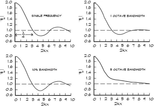
As the angle of incidence θ increases, the wavelength of the pattern also increases. Figures 7.3a, d, and g show the pressure patterns for angles of incidence of 0◦, 30◦, and 60◦.
Coherent Reflections—Random Incidence
When there is a reverberant field, the sound is incident on a boundary from any direction with equal probability, and the expression in Eq. 7.14 is averaged (integrated) over a hemisphere. This yields
p2r=[1+sin(2 k x)/2 k x] (7.15)
which is plotted in Fig. 7.3j.
The velocity plots in this figure are particularly interesting. Porous sound absorbing materials are most effective when they are placed in an area of high particle velocity. For normal incidence this is at a quarter wavelength from the surface. For off-axis and random incidence the maximum velocity is still at a quarter wavelength; however, there is some positive particle velocity even at the boundary surface that has a component perpendicular to the normal. Thus materials can absorb sound energy even when they are placed close to a reflecting boundary; however, they are more effective, particularly at low frequencies, when located away from the boundary.
Coherent Reflections—Random Incidence, Finite Bandwidth
When the sound is not a simple pure tone, there is a smearing of the peaks and valleys in the pressure and velocity standing waves. Both functions must be integrated over the bandwidth of the frequency range of interest.
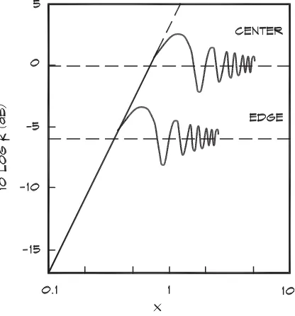
Figure7.5 Intensity vs Distance from a Reflecting Wall (Waterhouse, 1955)
The second term is a well-known tabulated integral. Figure 7.5 shows the result of the integration. Near the wall the mean-square pressure still exhibits a doubling (6 dB increase) and the particle velocity is zero.
7.2 REFLECTIONS FROM FINITE OBJECTS
Scattering from Finite Planes
Reflection from finite planar surfaces is of particular interest in concert hall design, where panels are frequently suspended as “clouds” above the orchestra. Usually these clouds are either flat or slightly convex toward the audience. A convex surface is more forgiving of imperfect alignment since the sound tends to spread out somewhat after reflecting.
If a sound wave is incident on a finite panel, there are several factors that influence the scattered wave. For high frequencies impacting near the center of the panel, the reflection is the same as that which an infinite panel would produce. Near the edge of the panel, diffraction (bending) can occur. Here the reflected amplitude is reduced and the angle of incidence may not be equal to the angle of reflection. At low frequencies, where the wavelength is much larger than the panel, the sound energy simply flows around it like an ocean wave does around a boulder.
Figure7.6 Geometry of the Reflection from a Finite Panel
Kirchoff-Fresnel approximation by Leizer (1966) or Ando (1985). The reflected intensity can be expressed as a diffraction coefficientKmultiplied times the intensity that would be reflected from a corresponding infinite surface. For a rectangular reflector the attenuation due to diffraction is
Ldif =10 logK =10 log(K1K2) (7.17)
where K =diffraction coefficient for a finite panel
K1 =diffraction coefficient for the x panel dimension K2 =diffraction coefficient for the y panel dimension
The orthogonal-panel dimensions can be treated independently. Rindel (1986) gives the coefficient for one dimension
K1 = 1
The terms C and S in Eq. 7.18 are the Fresnel integrals
Figure7.7 Attenuation of a Reflection Due to Diffraction (Rindel, 1986)
The integration limit v takes on the values of v1 or v2 according to the term of interest in Eq. 7.18. For everyday use these calculations are cumbersome. Accordingly we examine approximate solutions appropriate to regions of the reflector.
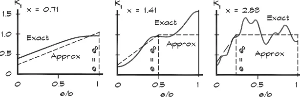
Rindel (1986) considers the special case of the center of the panel where e= b and v1 =v2 =x. Then Eq. 7.18 becomes
K1,center =2[C(x)]2+[S(x)]2
(7.22)
where
x=2b cosθ/√λa∗ (7.23)
and the characteristic distance a∗is
a∗=2 a1a2/ (a1 +a2) (7.24)
Figure 7.7 gives the value of the diffraction attenuation. At high frequencies where x>1, although there are fluctuations due to the Fresnel zones, a panel approaches zero diffraction attenuation as x increases. At low frequencies (x<0.7) the approximation
K1,center ∼=2 x2 for x<0.7 (7.25)
yields a good result.
At the edge of the panel where e=0, v1 =0, and v2 =2x we can solve for the value of the diffraction coefficient (Rindel, 1986)
K1,edge= 1 2
[C(2x)]2+[S(2x)]2
which is also shown in Fig. 7.7. The approximations in this case are
K1,edge ∼=2 x2 for x≤0.35 (7.27)
and
K1,edge ∼=1/4 for x>1 (7.28)
Based on these special cases Rindel (1986) divides the panel into three zones according to the nearness to the edge of the impact point
a) x ≤0.35:K1 ∼=2 x2, independent of the value of e.
, is a linear interpolation between
the edge and center values.
c) x >0.7: Here the concept of an edge zone is introduced whose width, eo, is given attenuation must be considered. Rindel (1986) gives
K1 ∼=
Figure 7.8 compares these approximate values to those obtained from a more detailed analysis.
Rindel (1986) also cites results of measurements carried out in an anechoic chamber using gated impulses, which are reproduced in Fig. 7.9. He concludes that for values of
Figure7.8 Calculated Values of K
Figure7.9 Measured and Calculated Attenuation of a Sound Reflection from a Square Surface (Rindel, 1986)
x greater than 0.7, edge diffraction is of minor importance. This corresponds to a limiting frequency
fg > c a ∗
2 S cosθ (7.31)
where S is the panel area. For a 2 m square panel the limiting frequency is about 360 Hz for a 45◦angle of incidence and a characteristic distance of 6 m, typical of suspended reflectors.
Panel Arrays
When reflecting panels are arrayed as in Fig. 7.10, the diffusion coefficients must account for multipanel scattering. The coefficient in the direction shown is (Finne, 1987 and Rindel, 1990)
K1 = 1 2
I
i=1
C(v1,i)−C(v2,i) 2
+
I
i=1
S(v1,i)−S(v2,i) 2
(7.32)
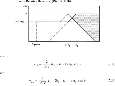
Figure7.11 Simplified Illustration of the Attenuation of Reflections from an Array with Relative Densityμ(Rindel, 1990)
where
v1,i = √2
λa∗(e1 −(i−1)m1)cos θ (7.33)
and
v2,i = √2
λa∗(e1−2b1 −(i−1)m1)cos θ (7.34)
whereiis the running row number andIis the total number of rows in the x-direction. At high frequencies the v values increase and the reflection is dominated by an indi-vidual panel. The single-panel limiting frequency from Eq. 7.31 sets the upper limit for this dependence. At low frequencies the v values decrease, but the reflected vectors combine in phase. The diffusion attenuation becomes dependent on the relative panel area density,μ, (the total array area divided by the total panel area), not the size of the individual reflectors. Figure 7.11 shows a design guide.
TheKvalues are approximately
K ∼=μ2 in the frequency range f
g,total ≤f ≤μfg (7.35)
where the limiting frequency for the total array is given by Eq. 7.31, with the total area of the array used instead of the individual panel area. The shaded area indicates the possible variation depending on whether the sound ray strikes a panel or empty space. Beranek (1992) published relative reflection data based on laboratory tests by Watters et al., (1963), which are shown in Fig. 7.12. In general a large number of small panels is preferable to a few large ones.
Bragg Imaging
Figure7.12 Scattering from Panel Arrays (Beranek, 1992)
of incidence. When two planes of reflectors are employed, for a given separation distance there is a relationship between the angle of incidence and the frequency of cancellation of the reflected sound. This effect was used by Bragg to study the crystal structure of materials with x-rays. When sound is scattered from two reflecting planes, certain frequencies are missing in the reflected sound. This was one cause of the problems in Philharmonic Hall in New York (Beranek, 1996).
An illustration of this phenomenon, known as Bragg imaging, is shown in Fig. 7.13. When two rows of reflecting panels are placed one above the other, there is destructive interference between reflected sound waves when the combined path-length difference has the relationship
2 d cos θ = (2 n−1) λ
2 (7.36)
where λ=wavelength of the incident sound (m or ft)
d=perpendicular spacing between rows of reflectors (m or ft) n=positive integer 1, 2, 3,. . .etc.
θ =angle of incidence and reflection with respect to the normal (rad or deg) The use of slightly convex reflectors can help diffuse the sound energy and smooth out the interferences; however, stacked planes of reflecting panels can produce a loss of bass energy in localized areas of the audience.
Scattering from Curved Surfaces
When sound is scattered from a curved surface, the curvature induces diffusion of the reflected energy when the surface is convex, or focusing when it is concave. The attenuation associated with the curvature can be calculated using the geometry shown in Fig. 7.14. If we consider a rigid cylinder having a radius R, the loss in intensity is proportional to the ratio of the incident-to-reflected beam areas (Rindel, 1986). At the receiver, M, the sound energy is proportional to the width of the reflected beam tube(a+a2)dβ. If there were no curvature the beam width would be(a1+a2)dβ1 at the image point M1.
Accordingly the attenuation due to the curvature is
Lcurv = −10 log (a+a2)dβ
and plugging this into Eq. 7.37 yields
Lcurv = −10 log
where a∗ is given in Eq. 7.24. For concave surfaces the same equation can be used with a negative value forR. Figure 7.15 shows the results for both convex and concave surfaces.
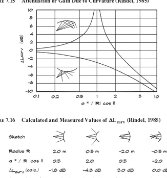
Figure7.15 Attenuation or Gain Due to Curvature (Rindel, 1985)
Figure7.16 Calculated and Measured Values ofL
curv (Rindel, 1985)
This analysis assumes that both the source and the receiver are in a plane whose normal is the axis of the cylinder. If this is not the case, both a∗ andθ must be deduced from a normal projection onto that plane (Rindel, 1985). Where there is a double-curved surface with two radii of curvature, the attenuation term must be applied twice, using the appropriate projections onto the two normal planes of the surface.
Figure 7.16 gives the results of measurements using TDS on a small (1.4 m×1.0 m) curved panel at a distance of 1 m for a zero angle of incidence over a frequency range of 3 to 19 kHz. The data also show the variation in the measured values, which Rindel (1985) attributes to diffraction effects.
Combined Effects
When sound is reflected from finite curved panels, the combined effects of distance, absorp-tion, size, and curvature must be included. For an omnidirectional source, the level of the reflected sound relative to the direct sound is
where the absorption term will be addressed later in this chapter, and the distance term is
Ldist =20 log a0
a1+a2 (7.41)
The other terms have been treated earlier.
Whispering Galleries
If a source of sound is located in a circular space, very close to the outside wall, some of the sound rays strike the surface at a shallow angle and are reflected again and again, and so propagate within a narrow band completely around the room. A listener located on the opposite side of the space can clearly hear conversations that occur close to the outside wall. This phenomenon, which is called a whispering gallery since even whispered conversations are audible, occurs in circular or domed spaces such as the statuary gallery in the Capital building in Washington, DC.
7.3 ABSORPTION
Reflection and Transmission Coefficients
When sound waves interact with real materials the energy contained in the incident wave is reflected, transmitted through the material, and absorbed within the material. The surfaces treated in this model are generally planar, although some curvature is tolerated as long as the radius of curvature is large when compared to a wavelength. The energy balance is illustrated in Fig. 7.17.
Ei =Er +Et+Ea (7.42)
Since this analysis involves only the interaction at the boundary of the material, the dif-ference between absorption, where energy is converted to heat, and transmission, where energy passes through the material, is not relevant. Both mechanisms are absorptive from the standpoint of the incident side because the energy is not reflected. Because we are only interested in the incident side of the boundary, we can combine the transmitted and
absorbed energies. If we divide Eq. 7.42 by Ei,
1= Er Ei +
Et+a
Ei (7.43)
We can express each energy ratio as a coefficient of reflection or transmission. The fraction of the incident energy that is absorbed (or transmitted) at the surface boundary is the coefficient
αθ = Et+a
Ei (7.44)
and the reflection coefficient is
αr = Er
Ei (7.45)
Substituting these coefficients into Eq. 7.43,
1=αθ +αr (7.46)
The reflection coefficient can be expressed in terms of the complex reflection amplitude ratio rfor pressure that was defined in Eq. 7.7
αr =r2 (7.47)
and the absorption coefficient is
αθ =1−r2 (7.48)
The reflected energy is
Er =(1−αθ)Ei (7.49)
Impedance Tube Measurements
When a plane wave is normally incident on the boundary between two materials, 1 and 2, we can calculate the strength of the reflected wave from a knowledge of their impedances. (This solution was published by Rayleigh in 1896.) Following the approach taken in Eq. 7.3, the sound pressure from the incident and reflected waves is written as
p(x)=Aej(ωt−k x)+Bej(ωt+k x) (7.50)
If we square and average this equation, we obtain the mean-squared acoustic pressure of a normally incident and reflected wave (Pierce, 1981)
Figure7.18 Impedance Tube Measurements of the Absorption Coefficient
The maximum value of the mean-squared pressure is12A2[1+ |r|]2, which occurs whenever 2 k x+δr is an even multiple ofπ. The minimum is 12 A2[1− |r|]2, which occurs at odd multiples of π. The ratio of the maximum-to-minimum pressures is an easily measured quantity called thestanding wave ratio, s, which is usually obtained from its square
s2 =
where xmin 1 is the smallest distance to a minimum and xmax 1 is the smallest distance to a maximum, measured from the surface of the material. The numbers m and n are arbitrary integers, which do not affect the relative phase. Equation 7.52 can be solved for the magnitude and phase of the reflection amplitude ratio
r= |r|ejδr (7.54)
from which the normal incidence material impedance can be obtained.
zn =ρ0c0(1+r)
(1−r) (7.55)
Oblique Incidence Reflections—Finite Impedance
When sound is obliquely incident on a surface having a finite impedance, the pressure of the incident and reflected waves is given by
p=A
and the velocity in the x direction at the boundary (x=0) using Eq. 6.31 is
The normal specific acoustic impedance, expressed as the ratio of the pressure to the velocity at the surface is
The reflection coefficient can then be written in terms of the boundary’s specific acoustic impedance
r= z−ρ0c0
z+ρ0c0 (7.59)
where z=zncosθ andzn =wn +jxn
z=complex specific acoustic impedance
=(pressure or force) / (particle or volume velocity)
w=specific acoustic resistance or real part of the impedance
x=specific acoustic reactance or the imaginary part of the impedance - when positive it is mass like and when negative it is stiffness like ρ0c0 =characteristic acoustic resistance of the incident medium
(about 412 Ns/m3- mks rayls in air) j=√−1
Now these relationships contain a good deal of information about the reflection process. When |z| ≫ ρ0c0 the reflection coefficient approaches a value of + 1, there is perfect reflection, and the reflected wave is in phase with the incident wave. If |z| ≪ ρ0c0, the boundary is resilient like the open end of a tube, and the value ofrapproaches−1. Here the reflected wave is 180◦out of phase with the incident wave and there is cancellation. When |z| =ρ0c0, no sound is reflected.
For any finite value of zn, as θ approaches π/2, the incident wave grazes over the boundary and the value ofrapproaches−1. Under this condition the incident and reflected waves are out of phase and interfere with one another. This is an explanation of the ground effect, which was discussed previously. Note that in both cases—that is, whenr is either± 1—there is no sound absorption by the surface. The|r| = −1 case is rarely encountered in architectural acoustics and only over limited frequency ranges (Kuttruff, 1973).
Reflection and transmission coefficients can also be written in terms of the normal acoustic impedance of a material. The energy reflection coefficient using Eq. 7.59 is
and in terms of the real and imaginary components of the impedance,
The absorption coefficient is set equal to the absorption/transmission coefficient given in Eq. 7.44, since it is defined at a surface where it does not matter whether the energy is transmitted through the material or absorbed within the material, as long as it is not reflected back. The specular absorption coefficient is
αθ =1−
which in terms of its components is
αθ = 4ρ0c0wncosθ #
wn cosθ +ρ0c0$2+x2 n cos2θ
(7.63)
For most architectural situations the incident conducting medium is air; however, it could be any material with a characteristic resistance. Since solid surfaces such as walls or absorptive panels have a resistancewn ≫ρ0c0, the magnitude of the absorption coefficient yields a maximum value whenwn cosθi = ρ0c0. For normal incidence, whenzn = ρ0c0, the transmission coefficient is unity as we would expect.
Figure 7.19 shows the behavior of a typical absorption coefficient with angle of inci-dence. As the angle of incidence increases, the apparent depth of the material increases, thereby increasing the absorption. At very high angles of incidence there is no longer a velocity component into the material so the coefficient drops off rapidly.
Figure7.20 Geometry of the Diffuse Field Absorption Coefficient Calculation (Cremer et al., 1982)
Calculated Diffuse Field Absorption Coefficients
In Eq. 7.63 we saw that we could write the absorption coefficient as a function of the angle of incidence, in terms of the complex impedance. Although direct-field absorption coefficients are useful for gaining an understanding of the physics of the absorption process, for most architectural applications a measurement is made of the diffuse-field absorption coefficient. Recall that a diffuse field implies that incident sound waves come from any direction with equal probability. The diffuse-field absorption coefficient is the average of the coefficientαθ, taken over all possible angles of incidence. The geometry is shown in Fig. 7.20. The energy from a uniformly radiating hemisphere that is incident on the surfaceSis proportional to the area that lies between the angleθ − θ/2 andθ + θ/2. The fraction of the total energy coming from this angle is
dE
and the total power sound absorbed by a projected area S cos θ is
W=E c S π/2
0
αθ sin θ cosθdθ (7.65)
The total incident power from all angles is the value of Eq. 7.65, with a perfectly absorptive material(αθ =1). The average absorption coefficient is the ratio of the absorbed to the total power
which can be simplified to (Paris, 1928)
α=2 π/2
0
Here the sine term is the probability that energy will originate at a given angle and the cosine term is the projection of the receiving area.
Measurement of Diffuse Field Absorption Coefficients
Although diffuse-field absorption coefficients can be calculated from impedance tube data, more often they are measured directly in a reverberant space. Values ofαare published for a range of frequencies between 125 Hz and 4 kHz. Each coefficient represents the diffuse-field absorption averaged over a band of frequencies one octave wide. Occasionally absorption data are required for calculations beyond this range. In these cases estimates can be made from impedance tube data, by extrapolation from known data, or by calculating the values from first principles.
Some variability arises in the measurement of the absorption coefficient. The diffuse-field coefficient is, in theory, always less than or equal to a value of one. In practice, when the reverberation time method discussed in Chapt. 8, is employed, values ofαgreater than 1 are sometimes measured. This normally is attributed to diffraction, the lack of a perfectly diffuse field in the measuring room, and edge conditions. At low frequencies diffraction seems to be the main cause (Beranek, 1971). Since it is easier and more consistent to measure the absorption using the reverberation time method, this is the value that is found in the published literature.
Diffuse-field measurements of the absorption coefficient are carried out in a reverber-ation chamber, which is a room with little or no absorption. Data are taken with and without the panel under test in the room and the resulting reverberation times are used to calculate the absorptive properties of the material. The test standard, ASTM C423, specifies several mountings as shown in Fig 7.21. Mountings A, B, D, and E are used for most prefabricated products. Mounting F is for duct liners and C is used for specialized applications. When data are reported, the test mounting method must also be included since the airspace behind the material greatly affects the results. The designation E-400, for example, indicates that mounting E was used and there was a 400 mm (16”) airspace behind the test sample.
Noise Reduction Coefficient (NRC)
Absorptive materials, such as acoustical ceiling tile, wall panels, and other porous absorbers are often characterized by their noise reduction coefficient, which is the average diffuse field absorption coefficient over the speech frequencies, 250 Hz to 2 kHz, rounded to the nearest 0.05.
NRC= 1 4 #
α250+α500+α1 k+α2 k$ (7.68)
Although these single-number metrics are useful as a means of getting a general idea of the effectiveness of a particular material, for critical applications calculations should be carried out over the entire frequency range of interest.
Absorption Data
Figure7.21 Laboratory Absorption Test Mountings
of the measured data, some adjustments may have to be made to account for different air cavity depths or mounting methods.
Occasionally it is necessary to estimate the absorption of materials beyond the range of measured data. Most often this occurs in the 63 Hz octave band, but sometimes occurs at lower frequencies. Data generally are not measured in this frequency range because of the size of reverberant chamber necessary to meet the diffuse field requirements. In these cases it is particularly important to consider the contributions to the absorption of the structural elements behind any porous panels.
Layering Absorptive Materials
It is the rule rather than the exception that acoustical materials are layered in real applications. For example a 25 mm (1 in) thick cloth-wrapped fiberglass material might be applied over a 16 mm (5/8 in) thick gypsum board wall. A detailed mathematical analysis of the impedance of the composite material is beyond the scope of a typical architectural project, and when one seeks the absorption coefficient from tables such as those in Table 7.1, one finds data on the panel, tested in an A-mounting condition, and data on the gypsum board wall, but no data on the combination.
Table7.1 Absorption Coefficients of Common Materials
Material Mount Frequency, Hz
125 250 500 1k 2k 4k
Walls
Glass, 1/4”, heavy plate 0.18 0.06 0.04 0.05 0.02 0.02
Glass, 3/32”, ordinary window 0.55 0.25 0.18 0.12 0.07 0.04
Gypsum board, 1/2”, 0.29 0.10 0.05 0.04 0.07 0.09
on 2×4 studs
Plaster, 7/8”, gypsum or 0.013 0.015 0.02 0.03 0.04 0.05
lime, on brick
Plaster, on concrete block 0.12 0.09 0.07 0.05 0.05 0.04
Plaster, 7/8”, on lath 0.14 0.10 0.06 0.04 0.04 0.05
Plaster, 7/8”, lath on studs 0.30 0.15 0.10 0.05 0.04 0.05
Plywood, 1/4”, 3” air 0.60 0.30 0.10 0.09 0.09 0.09
space, 1” batt,
Soundblox, type B, painted 0.74 0.37 0.45 0.35 0.36 0.34
Wood panel, 3/8”, 3-4” air 0.30 0.25 0.20 0.17 0.15 0.10
space
Concrete block, unpainted 0.36 0.44 0.51 0.29 0.39 0.25
Concrete block, painted 0.10 0.05 0.06 0.07 0.09 0.08
Concrete poured, unpainted 0.01 0.01 0.02 0.02 0.02 0.03
Brick, unglazed, unpainted 0.03 0.03 0.03 0.04 0.05 0.07
Wood paneling, 1/4”, 0.42 0.21 0.10 0.08 0.06 0.06
with airspace behind
Wood, 1”, paneling with 0.19 0.14 0.09 0.06 0.06 0.05
airspace behind
Shredded-wood A 0.15 0.26 0.62 0.94 0.64 0.92
fiberboard, 2”, on concrete
Carpet, heavy, on 5/8-in 0.37 0.41 0.63 0.85 0.96 0.92
perforated mineral fiberboard
Brick, unglazed, painted A 0.01 0.01 0.02 0.02 0.02 0.03
Light velour, 10 oz per sq 0.03 0.04 0.11 0.17 0.24 0.35
yd, hung straight, in contact with wall
Medium velour, 14 oz per 0.07 0.31 0.49 0.75 0.70 0.60
sq yd, draped to half area
Heavy velour, 18 oz per sq 0.14 0.35 0.55 0.72 0.70 0.65
yd, draped to half area
Table7.1 Absorption Coefficients of Common Materials, (Continued)
Material Mount Frequency, Hz
125 250 500 1k 2k 4k
Floors
Floors, concrete or terrazzo A 0.01 0.01 0.015 0.02 0.02 0.02
Floors, linoleum, vinyl on A 0.02 0.03 0.03 0.03 0.03 0.02
concrete
Floors, linoleum, vinyl on 0.02 0.04 0.05 0.05 0.10 0.05
subfloor
Floors, wooden 0.15 0.11 0.10 0.07 0.06 0.07
Floors, wooden platform 0.40 0.30 0.20 0.17 0.15 0.10
w/airspace
Carpet, heavy on concrete A 0.02 0.06 0.14 0.57 0.60 0.65
Carpet, on 40 oz (1.35 A 0.08 0.24 0.57 0.69 0.71 0.73
kg/sq m) pad
Indoor-outdoor carpet A 0.01 0.05 0.10 0.20 0.45 0.65
Wood parquet in asphalt A 0.04 0.04 0.07 0.06 0.06 0.07
on concrete
Acoustical coating K-13 A 0.12 0.38 0.88 1.16 1.15 1.12
“fc” 1”
Glass-fiber roof fabric, 12 0.65 0.71 0.82 0.86 0.76 0.62
oz/yd
Glass-fiber roof fabric, 0.38 0.23 0.17 0.15 0.09 0.06
37.5 oz/yd
Acoustical Tile
Standard mineral fiber, E400 0.68 0.76 0.60 0.65 0.82 0.76
5/8”
Standard mineral fiber, E400 0.72 0.84 0.70 0.79 0.76 0.81
3/4”
Standard mineral fiber, 1” E400 0.76 0.84 0.72 0.89 0.85 0.81
Energy mineral fiber, 5/8” E400 0.70 0.75 0.58 0.63 0.78 0.73
Energy mineral fiber, 3/4” E400 0.68 0.81 0.68 0.78 0.85 0.80
Energy mineral fiber, 1” E400 0.74 0.85 0.68 0.86 0.90 0.79
Film faced fiberglass, 1” E400 0.56 0.63 0.69 0.83 0.71 0.55
Film faced fiberglass, 2” E400 0.52 0.82 0.88 0.91 0.75 0.55
Film faced fiberglass, 3” E400 0.64 0.88 1.02 0.91 0.84 0.62
Table7.1 Absorption Coefficients of Common Materials, (Continued)
Material Mount Frequency, Hz
125 250 500 1k 2k 4k
Glass Cloth Acoustical Ceiling Panels
Fiberglass tile, 3/4” E400 0.74 0.89 0.67 0.89 0.95 1.07
Fiberglass tile, 1” E400 0.77 0.74 0.75 0.95 1.01 1.02
Fiberglass tile, 1 1/2” E400 0.78 0.93 0.88 1.01 1.02 1.00
Seats and Audience
Audience in upholstered seats 0.39 0.57 0.80 0.94 0.92 0.87
Unoccupied well- 0.19 0.37 0.56 0.67 0.61 0.59
upholstered seats
Unoccupied leather 0.19 0.57 0.56 0.67 0.61 0.59
covered seats
Wooden pews, occupied 0.57 0.44 0.67 0.70 0.80 0.72
Leather-covered upholstered 0.44 0.54 0.60 0.62 0.58 0.50
seats, unoccupied
Congregation, seated in 0.57 0.61 0.75 0.86 0.91 0.86
wooden pews
Chair, metal or wood seat, 0.15 0.19 0.22 0.39 0.38 0.30
unoccupied
Students, informally 0.30 0.41 0.49 0.84 0.87 0.84
dressed, seated in
tablet-Aeroflex Type 150, 1” F 0.13 0.51 0.46 0.65 0.74 0.95
Aeroflex Type 150, 2” F 0.25 0.73 0.94 1.03 1.02 1.09
Aeroflex Type 200, 1/2” F 0.10 0.44 0.29 0.39 0.63 0.81
Aeroflex Type 200, 1” F 0.15 0.59 0.53 0.78 0.85 1.00
Aeroflex Type 200, 2” F 0.28 0.81 1.04 1.10 1.06 1.09
Aeroflex Type 300, 1/2” F 0.09 0.43 0.31 0.43 0.66 0.98
Aeroflex Type 300, 1” F 0.14 0.56 0.63 0.82 0.99 1.04
Aeroflex Type 150, 1” A 0.06 0.24 0.47 0.71 0.85 0.97
Aeroflex Type 150, 2” A 0.20 0.51 0.88 1.02 0.99 1.04
Aeroflex Type 300, 1” A 0.08 0.28 0.65 0.89 1.01 1.04
Table7.1 Absorption Coefficients of Common Materials, (Continued)
Material Mount Frequency, Hz
125 250 500 1k 2k 4k
Building Insulation -Fiberglass
3.5” (R-11) (insulation A 0.34 0.85 1.09 0.97 0.97 1.12
exposed to sound)
6” (R-19) (insulation A 0.64 1.14 1.09 0.99 1.00 1.21
exposed to sound)
3.5” (R11) (FRK facing A 0.56 1.11 1.16 0.61 0.40 0.21
exposed to sound)
FB, FRK faced, 1” thick E400 0.48 0.60 0.80 0.82 0.52 0.35
FB, FRK faced, 2” thick E400 0.50 0.61 0.99 0.83 0.51 0.35
FB, FRK faced, 3” thick E400 0.59 0.64 1.09 0.81 0.50 0.33
FB, FRK faced, 4” thick E400 0.61 0.69 1.08 0.81 0.48 0.34
Miscellaneous
Musician (per person), 4.0 8.5 11.5 14.0 15.0 12.0
with instrument
Air, Sabins per 1000 cubic 0.9 2.3 7.2
In cases where materials are applied in ways that differ from the manner in which they were tested, estimates must be made based on the published absorptive properties of the individual elements. For example, a drywall wall has an absorptive coefficient of 0.29 at 125 Hz since it is acting as a panel absorber, having a resonant frequency of about 55 Hz. A one-inch (25 mm) thick fiberglass panel has an absorption coefficient of 0.03 at 125 Hz since it is measured in the A-mounting position. When a panel is mounted on drywall, the low-frequency sound passes through the fiberglass panel and interacts with the drywall surface. Assuming the porous material does not significantly increase the mass of the wall surface, the absorption at 125 Hz should be at least 0.29, and perhaps a little more due to the added flow resistance of the fiberglass. Consequently when absorptive materials are layered we must consider the combined result, rather than the absorption coefficient of only the surface material alone.
7.4 ABSORPTION MECHANISMS
Absorptive materials used in architectural applications tend to fall into three categories: porous absorbers, panel absorbers, and resonant absorbers. Of these, the porous absorbers are the most frequently encountered and include fiberglass, mineral fiber products, fiberboard, pressed wood shavings, cotton, felt, open-cell neoprene foam, carpet, sintered metal, and many other products. Panel absorbers are nonporous lightweight sheets, solid or perforated, that have an air cavity behind them, which may be filled with an absorptive material such as fiberglass. Resonant absorbers can be lightweight partitions vibrating at their mass-air-mass resonance or they can be Helmholtz resonators or other similar enclosures, which absorb sound in the frequency range around their resonant frequency. They also may be filled with absorbent porous materials.
Porous Absorbers
Several mechanisms contribute to the absorption of sound by porous materials. Air motion induced by the sound wave occurs in the interstices between fibers or particles. The move-ment of the air through narrow constrictions, as illustrated in Fig. 7.22, produces losses of momentum due to viscous drag (friction) as well as changes in direction. This accounts for most of the high-frequency losses. At low frequencies absorption occurs because fibers are relatively efficient conductors of heat. Fluctuations in pressure and density are isothermal, since thermal equilibrium is restored so rapidly. Temperature increases in the gas cause heat
to be transported away from the interaction site to dissipate. Little attenuation seems to occur as a result of induced motion of the fibers (Mechel and Ver, 1992).
A lower (isothermal) sound velocity within a porous material also contributes to absorp-tion. Friction forces and direction changes slow down the passage of the wave, and the isothermal nature of the process leads to a different equation of state. When sound waves travel parallel to the plane of the absorber some of the wave motion occurs within the absorber. Waves near the surface are diffracted, drawn into the material, due to the lower sound velocity.
In general, porous absorbers are too complicated for their precise impedances to be predicted from first principles. Rather, it is customary to measure the flow resistance, rf, of the bulk material to determine the resistive component of the impedance. The bulk flow resistance is defined as the ratio between the pressure drop P across the absorbing material and the steady velocity usof the air passing through the material.
rf = − P
us (7.69)
Since this is dependent on the thickness of the absorber it is not a fundamental property of the material. The material property is thespecific flow resistance, rs, which is independent of the thickness.
rs = −1 us
P x =
rf
x (7.70)
Flow resistance can be measured (Ingard, 1994) using a weighted piston as in Fig. 7.23. When the piston reaches its steady velocity, the resistance can be determined by measuring the time it takes for the piston to travel a given distance and the mass of the piston. Flow resistance is expressed in terms of the pressure drop in Newtons per square meter divided by the velocity in meters per second and is given in units of mks rayls, the same unit as the specific acoustic impedance. The specific flow resistance has units of mks rayls/m.
Figure7.24 Geometry of a Spaced Porous Absorber (Kuttruff, 1973)
Spaced Porous Absorbers—Normal Incidence, Finite Impedance
If a thin porous absorber is positioned such that it has an airspace behind it, the composite impedance at the surface of the material and thus the absorption coefficient, is influenced by the backing. Figure 7.24 shows a porous absorber located a distance d away from a solid wall. The flow resistance, which is approximately the resistive component of the impedance, is the difference in pressure across the material divided by the velocity through the material.
rf = p1−p2
u (7.71)
wherep1 is the pressure on the left side of the sheet andp2 is the pressure just to the right of the sheet. In this analysis it is assumed that the resistance is the same for steady and alternating flow. The velocity on either side of the sheet is the same due to conservation of mass. Equation 7.71 can be written in terms of the impedance at the surface of the absorber (at x=0) on either side of the sheet.
rf =z1−z2 (7.72)
which implies that the impedance of the composite sheet plus the air backing is the sum of the sheet flow resistance and the impedance of the cavity behind the absorber.
z1 =rf +z2 (7.73)
To calculate the impedance of the air cavity for a normally incident sound wave we write the equations for a rightward moving wave and the reflected leftward moving wave, assuming perfect reflection from the wall.
p2(x)=A"e−j k(x−d)+ej k(x−d)%
=2Acos"
The velocity in the cavity is
The ratio of the pressure to the velocity at the sheet surface (x = 0) is the impedance of the cavity
The normal impedance of the porous absorber and the air cavity is
zn =rf −jρ0c0 cot(k d) (7.77)
By plugging this expression into Eq. 7.63 we get the absorption coefficient for normal incidence (Kuttruff, 1973)
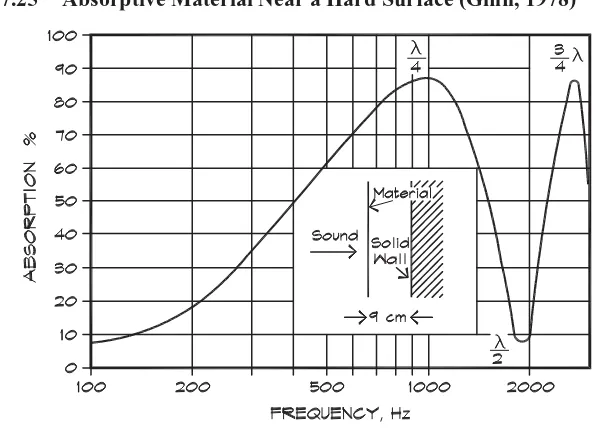
Figure 7.25 (Ginn, 1978) shows the behavior of this equation with frequency for a flow resistance rf ∼=2ρ0c0.
A thin porous absorber located at multiples of a quarter wavelength from a reflecting surface is in an optimum position to absorb sound since the particle velocity is at a maximum at this point. An absorber located at multiples of one-half wavelength from a wall is not particularly effective since the particle velocity is low. Thin curtains are not good broadband absorbers unless there is considerable (usually 100%) gather or unless there are several curtains hung one behind another. Note that in real rooms it is rare to encounter a condition of purely normal incidence. For diffuse fields the phase interference patterns are much less pronounced than those shown in Fig. 7.25.
Porous Absorbers with Internal Losses—Normal Incidence
When there are internal losses that attenuate the sound as it passes through a material, the attenuation can be written as an exponentially decaying sinusoid
p(x)=Aejωte−jqx (7.79)
whereq = δ+jβ is the complexpropagation constantwithin the absorbing material. It is much like the wave number in that its real part, δ, is close toω/c. However, it has an imaginary part,β, which is the attenuation constant, in nepers/meter, of the sound passing through an absorber. To convert nepers per meter to dB/meter, multiply nepers by 8.69.
For a thick porous absorber with a characteristic wave impedancezw, we write the equations for a normally incident and reflected plane wave with losses
p=Aejqx+Be−jqx (7.80)
and the particle velocity is
u= 1 zw
Aejqx−Be−jqx (7.81)
We use the indices 1 and 2 for the left- and right-hand sides of the material and make the end of the material x=0 and the beginning of the material x= −d. The incident wave is moving in the positive x direction. At x=0,
p2 =A+B (7.82)
and
u2 = 1
zw(A−B) (7.83)
Solving for the amplitudes A and B,
A=(p2+zw u2) /2 (7.84)
B=(p2−zw u2) /2 (7.85)
Plugging these into Eqs. 7.80 and 7.81 at x= −d,
and
The ratio of these two equations yields the input impedance of the absorbing surface in terms of the characteristic wave impedance of the material and its propagation constant, and the back impedancez2 of the surface behind the absorber.
z1 =zw
Empirical Formulas for the Impedance of Porous Materials
It is difficult to predict the complex characteristic impedance of a material from the flow resistance based on theory alone, so empirical formulas have been developed that give good results. Delany and Bazley (1969) published a useful relationship for the wave impedance of a porous material such as fiberglass
zw =w+jx (7.90)
and the propagation constant is
q=δ+jβ (7.93)
where zw =complex characteristic impedance of the material w=resistance or real part of the wave impedance
x=reactance or imaginary part of the wave impedance q=complex propagation constant
δ=real part of the propagation constant∼=ω/c0
ρ0c0 =characteristic acoustic resistance of air (about 412 Ns/m3−mks rayls)
rs =specific flow resistance (mks rayls) d=thickness of the material (m) f =frequency (Hz)
j=√−1
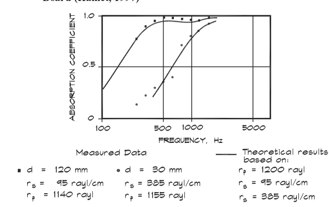
Figure 7.26 shows measured absorption data versus frequency compared to calculated data using the relationships just shown for two different flow resistance and thickness values. Note that manufacturers usually give the specific flow resistance in cgs rayls/cm (1 cgs rayl=10 mks rayls). The shape of the curve is determined by the total flow resistance, and the thickness sets the cutoff point for low-frequency absorption.
Diffuse-field absorption coefficients show a similar behavior with thickness. For oblique incidence there is a component of the velocity parallel to the surface so there is some absorption, even near the wall. The thickness and spacing of a porous absorber such as a pressed-fiberglass panel, mounted on a concrete wall or other highly reflecting surface, still determines the frequency range of its absorption characteristics. Figure 7.27 shows the measured diffuse-field absorption coefficients of various thicknesses of felt panel.
Thick Porous Materials with an Air Cavity Backing
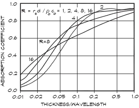
When a thick porous absorber is backed by an air cavity and then a rigid wall, the back impedance behind the absorber is given in Eq. 7.76. This value can be inserted into Eq. 7.63 to get the overall impedance of the composite. The absorption coefficient is plotted in Fig. 7.28 for several thicknesses. In each case the total depth and total flow resistance are the same. Note that the specific flow resistance has been changed to offset the changes in thickness. When materials are spaced away from the wall, they should have a higher characteristic resistance. It is interesting that, as the material thickness decreases, the effect of the quarter-wave spacing becomes more noticeable since its behavior approaches that of a thin resistive absorber.
Figure7.27 Dependence of Absorption on Thickness (Ginn, 1978)
Figure7.28 Absorption of Thick Materials with Air Backing (Ingard, 1994)
Practical Considerations in Porous Absorbers
Figure7.29 Diffuse Field Absorption Coefficient (Ingard, 1994)
Figure 7.29 shows the absorption of materials of the same thickness but having different flow resistances. Normally a value around 2ρ0c0 of total flow resistance is optimal at the mid and high frequencies for a wall-mounted absorber (Ingard, 1994). At lower frequencies, or when there is an air cavity backing, higher resistances are better.
When a relatively dense material such as acoustical tile is suspended over an airspace, it can be an effective broadband absorber. Figure 7.30 shows the difference in low-frequency performance for acoustical tiles applied with adhesive directly to a reflecting surface and those supported in a suspension system. The thickness of the material is still important so that the absorption coefficient does not exhibit the high-frequency dependence shown earlier. In general, fiberglass tiles are more effective at high frequencies than mineral-fiber tiles since their characteristic resistance is lower.
Wrapping materials with a porous cloth covering has little effect on the absorption coefficient. The flow resistance of the cloth must be low. If it is easy to blow through it there is little change in the absorption. Paper or vinyl backings raise the resistance and lower the high-frequency absorption. Small perforations made in a vinyl fabric can reduce the flow resistance while delivering a product that is washable.
Screened Porous Absorbers
Figure7.30 Average Absorption of Acoustical Tiles (Doelle, 1972)
Figure7.31 Sound Absorption of Perforated Panels (Doelle, 1972)
Figure7.32 Various Configurations of Wood Slats (Doelle, 1972)
Figure7.33 Effect of Paint on Absorptive Panels (Doelle, 1972)
7.5 ABSORPTION BY NONPOROUS ABSORBERS
Unbacked Panel Absorbers
Figure7.34 Geometry of an Unbacked Panel Absorber
into free space we can write the pressure in terms of the particle velocity p2 = ρ0c0uto obtain the relationshipp1+p3−ρ0c0u=jωmuand from this, the impedance of the panel is (Kuttruff, 1963)
z=jωm+ρ0c0 (7.96)
Now this expression can be inserted into Eq. 7.63 to calculate the normal incidence absorption coefficient
αn = ⎡
⎣1+ '
ωm 2ρ0c0
(2⎤
⎦ −1
(7.97)
From this expression the absorption of windows and solid walls can be calculated; however, their residual absorption is small and only significant at low frequencies.
Air Backed Panel Absorbers
When a nonporous panel, as in Fig. 7.35, is placed in front of a solid surface with no contact between the panel and the surface, the panel can move back and forth, but is resisted by the air spring force.
When there is a pressure differential across the panel Newton’s law governs the motion
p=mdu
d t =jωmu (7.98)
where m is the mass of the panel per unit area. Using the same notation as before, with p1+p3 being the pressure in front of the panel andp2 the pressure behind the absorber, we obtain
p1 +p3 −p2
u =rf +jωm (7.99)
and in a similar manner the composite assembly impedance is
z=rf +j"ωm−ρ0c0 cot(k d)% (7.100)
When the depth, d, of the airspace behind the sheet is small compared to a wavelength, we can use the approximation cot(k d)∼=(k d)−1so that
As before, we can insert this expression into Eq. 7.63 to obtain the normal-incidence absorption coefficient (Kuttruff, 1973)
where we have used the resonant frequency from the bracketed term in Eq. 7.101, whose terms are equal at resonance.
ωr =
A simpler version of Eq. 7.103 is
fr = √600
m d (7.104)
where m is the panel mass in kg/m2and d is the thickness of the airspace in cm. When the airspace is filled with batt insulation the resonant frequency is reduced to
fr = √500
m d (7.105)
due to the change in sound velocity.
Figure7.36 Sound Absorption of a Suspended Panel (Doelle, 1972)
off. In this model the sharpness of the peak is determined by the amount of flow resistance provided by the panel. When damping is added to the cavity the propagation constant in the airspace becomes complex and adds a real part to the impedance, which broadens the resonance. The damping is provided by fiberglass boards or batting suspended in the airspace behind the panel. Figure 7.36 shows the typical behavior of a panel absorber with and without insulation.
Panel absorbers of this type that are tuned to a low resonant frequency are used as bass traps in studios and control rooms. Thin wood panels, mounted over an air cavity, produce considerable low-frequency absorption and, when there is little or no absorptive treatment behind the panel, this absorption is frequently manifest in narrow bands. As a result wood panels are a serious detriment to adequate bass response in concert halls. It is a common misunderstanding, particularly among musicians, that wood, and in particular thin wood panels that vibrate, contribute to good acoustical qualities of the hall. This no doubt arises from the connection in the mind between a musical instrument such as a violin and the hall itself. In fact, vibrating components in a hall tend to remove energy at their natural frequencies and return some of it back to the hall at a later time.
Perforated Panel Absorbers
If a perforated plate is suspended in a sound field, there is absorption due to the mass reactance of the plate itself, the mass of the air moving through the perforations, and the flow resistance of the material. If the perforated plate is mounted over an air cavity, there is also its impedance to be considered. There are quite a number of details in the treatment of this subject, whose consideration extends past the scope of this book. The goal here is to present enough detail to give an understanding of the phenomena without undue mathematical complication.
Figure7.37 Geometry of a Perforated Panel Absorber
is forced through the holes. The ratio of velocities can be written in terms of the ratio of the areas, which is the porosity
ue ui =
πa2
e2 =σ (7.106)
The impedance due to the inertial mass of the air moving through the pores is
p1 −p2 ue =
jω πa2ρ0l
e2 =
jω ρ0l
σ (7.107)
so the effective mass per unit area is
m= ρ0l
σ (7.108)
The effective length of the tube made by the perforated hole in Eq. 7.107 is slightly longer than the actual thickness of the panel. This is because the air in the tube does not instantaneously accelerate from the exterior velocity to the interior velocity. There is an area on either side of the plate that contains a region of higher velocity and thus a slightly longer length. This correction is written in terms of the effective length
l=l0+2(0.8 a) (7.109)
Usually the air mass is very small compared to the mass of the panel itself so that the panel is not affected by the motion of the fluid. If the area of the perforations is large and the panel mass M is small, the combined mass of the air and the panel must be used.
mc =m M
M+m (7.110)
When M is large compared with the mass of the air, m, then the combined mass is just the air mass.
Figure7.38 Absorption of a Coated Perforated Panel (Wilhelmi Corp. Data, 2000)
metal sheets are available with an air resistant coating, which adds flow resistance to the mass reactance of the air. These materials can be supported by T-bar systems and are effective absorbers. Absorption data for a typical product are shown in Fig. 7.38.
Perforated Metal Grilles
When a perforated panel is being used as a grille to provide a transparent cover for a porous absorber, it is important that there is sufficient open area that the sound passage is not blocked. In these cases the sound “absorbed” by the panel is actually the sound transmitted through the grille into the space beyond. The normal incidence absorption coefficient in this case is the same as the normal incidence transmissivity. Thus we can set it equal to the expression shown in Eq. 7.97
τ = ⎡
⎣1+ '
ωmc 2ρ0c0
(2⎤
⎦ −1
(7.111)
If the loss through a perforated panel is to be less than about 0.5 dB, the transmission coefficient should be greater than about 0.9, and the term inside the parenthesis becomes 0.33. At 1000 Hz the combined panel mass should be 0.04 kg/m2. For a 2 mm thick (.079”) thick panel with 3 mm (.125”) diameter holes, the effective length is about 4 mm and the required porosity calculates out to about 11%. This compares well with the data shown in Fig. 7.38, even though the calculation done here is for normal incidence and the data are for a diffuse-field measurement.
If a perforated panel is to be used as a loudspeaker grille, the open area should be greater, on the order of 30 to 40%. Increasing the porosity preserves more of the off-axis directional character of the loudspeaker’s sound. Porosities beyond 40% are difficult to achieve in a perforated panel while still retaining structural integrity.
Air Backed Perforated Panels
frequencies was given in Eq. 7.102
z=jωmc + rf −jρ0c 2 0
ωd (7.112)
In the case of a perforated panel the combined mass of the panel and the air through the pores is used. We obtain the same result as Eq. 7.102, which we used for the absorption coefficient of a closed panel, and it is expressed in terms of the resonant frequency of the panel-cavity-spring-mass system.
When we substitute the mass of the moving air in terms of the length of the tube and the porosity we get a familiar result—the Helmholtz resonator natural frequency. Here we have assumed that the mass of the air is much smaller than the panel mass
mc= ρ0l
It is apparent that a perforated panel with an air backing is acting like a Helmholtz resonator absorber and will exhibit similar characteristics, just as the solid panel did. The major difference is that the moving mass, in this case the air in the holes, is much lighter than the panel and thus the resonant frequency is much higher. These perforated absorbers are mainly utilized where mid-frequency absorption is needed.
The flow resistance of perforated panels can be measured directly or can be calculated from empirical formulas, such as that given by Cremer and Muller (1982)
rf ∼=0.53 e
Figure 7.39 shows the absorption coefficient of a perforated plate in front of an airspace filled with absorptive material.
7.6 ABSORPTION BY RESONANT ABSORBERS
Helmholtz Resonator Absorbers
Figure7.39 Absorption of a Perforated Panel (Cremer and Muller, 1982)
The resonant frequency is given by
f0 = c0
where a is the radius of the resonator neck,l0 is its length, and V its volume. The question then is how to calculate the depth, d, of the cavity. With a perforated plate the volume of the airspace was
d = V
e2 (7.118)
where e is the spacing between perforations. Using V as the volume of the Helmholtz resonator the normal-incidence absorption coefficient for a series of resonators is (Cremer and Muller, 1982)
Products based on the Helmholtz resonator principle are commercially available. Some are constructed as concrete masonry units with slotted openings having a fibrous or metallic septum interior fill. Absorption data on typical units are given in Fig. 7.40.
Mass-Air-Mass Resonators
A mass-air-mass resonant system is one in which two free masses are separated by an air cavity that provides the spring force between them. A typical example is a drywall stud wall, which acts much like the resonant panel absorber, except that both sides are free to move. The equation is similar to that used in the single-panel equation (Eq. 7.104) except that both masses are included. The resonant frequency is
fmam =600 )
m1 +m2
d m1 m2 (7.120)
Figure7.40 Helmholtz Resonator Absorbers (Doelle, 1972)
the constant changes from 600 to 500 because the sound velocity goes from adiabatic to isothermal. Away from resonance the absorption coefficient follows the relationship (Bradley, 1997)
α(f)=αmam
fmam f
2
+αs (7.121)
where α(f)=diffuse field absorption coefficient αmam =maximum absorption coefficient at fmam
αs =residual surface absorption coefficient at high frequencies f =frequency (Hz)
fmam =mass-air-mass resonant frequency (Hz)
Figure 7.41 shows the absorption coefficient for a single and double-layer drywall stud wall usingαmam = 0.44 and αs = 0.045 for the single-layer wall andαmam = 0.44 and αs = 0.06 in the double-layer case. The same constants are used for batt-filled stud walls. The agreement shown in the figure between measured and predicted values is quite good.
Quarter-Wave Resonators
A hard surface having a well of depth d and diameter 2 a can provide absorption through reradiation of sound that is out of phase with the incident sound. These wells, shown in Fig. 7.42, are known as quarter-wave resonators because a wave reflected from the bottom returns a half wavelength or 180◦ out of phase with the wave reflected from the surface. When the length of the tube is an odd-integer multiple of a quarter wavelength it is out of phase with the incident wave and perfectly absorbing. The tube acts as a small resonant radiator, which can have both absorptive and diffusive properties.
As was the case in Eq. 7.89, the interaction impedance of a tube having a depth d is
Figure7.41 Resonant Absorption by a Stud Wall (Bradley, 1997)
Figure7.42 Quarter Wave Resonator
whereqis the propagation constant. The tube has small viscous and thermal loss components and the imaginary part of the propagation constant, from an approximation originally due to Kirchoff, can be used to account for them
q∼=k
-1+ 0.31 j 2 a√f
.
(7.123)
There are two impedances to be included in the analysis: one having to do with the interaction between the incoming wave and the end of the tube, which was given in Eq. 7.122; and the other having to do with the radiation of sound back out of the tube. The radiation impedance of the tube is that of a piston in a baffle and was examined in Eq. 6.67 and 6.69 in the near field. For low frequencies, where the width of the opening is much smaller than a wavelength, the radiation impedance is approximately (Morse, 1948)
zr ∼=ρ0c0
-1 2(k a)
2
+ 2 j
πk a .
(7.124)
Figure7.43 Absorption and Scattering Cross Sections of a Tube Resonator in a Wall (Ingard, 1994)
surface,poutside = 2pi +pr wherepr = u zr. The pressure just outside the opening must match the pressure just inside the end of the tube, which ispinside = −u zt. At the surface the pressures and the velocities must match, which leads to
u= 2pi zt +zr
(7.125)
The absorption of a well in a surface can be expressed in terms of a cross section, defined (Ingard, 1994) as the power absorbed by the well divided by the intensity of the incident wave. The power absorbed by the resonator tube is
Wa =S|u|2 wt =S
is the intensity of the incident wave, the power absorbed can be expressed as Wa =AaIi, where Aais the absorption cross section.
A typical result, given in Fig. 7.43, shows strong peaks at the minima of the tube impedance. When the cross section is 100, it means that the tube is acting as a perfect absorber equal to 100 times its open area. Note that although a tube can be very effective at a given frequency, its bandwidth is very narrow.