Publikasi - Bappeda Kab. Probolinggo

Android

Deep Dive Series

Zigurd Mednieks, Series Editor

The Android Deep Dive Series is for intermediate and expert developers who use Android Studio and Java, but do not have comprehensive knowledge of Android system-level programming or deep knowledge of Android APIs. Readers of this series want to bolster their knowledge of fundamentally important topics.

Each book in the series stands alone and provides expertise, idioms, frameworks, and engineering approaches. They provide in-depth information, correct patterns and idioms, and ways of avoiding bugs and other problems. The books also take advantage of new Android releases, and avoid deprecated parts of the APIs.

About the Series Editor

Android

Database Best

Practices

Adam Stroud

Boston฀•฀Columbus฀•฀Indianapolis฀•฀New฀York฀•฀San฀Francisco฀•฀Amsterdam฀•฀Cape฀Town Dubai฀•฀London฀•฀Madrid฀•฀Milan฀•฀Munich฀•฀Paris฀•฀Montreal฀•฀Toronto฀•฀Delhi฀•฀Mexico฀City

capital letters or in all capitals.

The author and publisher have taken care in the preparation of this book, but make no expressed or implied warranty of any kind and assume no responsibility for errors or omissions. No liability is assumed for incidental or consequential damages in connection with or arising out of the use of the information or programs contained herein.

For information about buying this title in bulk quantities, or for special sales opportunities (which may include electronic versions; custom cover designs; and content particular to your business, training goals, marketing focus, or branding interests), please contact our corporate sales department at corpsales@pearsoned.com or (800) 382-3419. For government sales inquiries, please contact governmentsales@pearsoned.com. For questions about sales outside the U.S., please contact intlcs@pearson.com. Visit us on the Web: informit.com/aw

Library of Congress Control Number: 2016941977 Copyright © 2017 Pearson Education, Inc.

All rights reserved. Printed in the United States of America. This publication is protected by copyright, and permission must be obtained from the publisher prior to any prohibited reproduction, storage in a retrieval system, or transmission in any form or by any means, electronic, mechanical, photocopying, recording, or likewise. For information regarding permissions, request forms and the appropriate contacts within the Pearson Education Global Rights & Permissions Department, please visit www.pearsoned.com/permissions/. The following are registered trademarks of Google: Android™, Google Play™.

Google and the Google logo are registered trademarks of Google Inc., used with permission.

The following are trademarks of HWACI: SQLite, sqlite.org, HWACI. Gradle is a trademark of Gradle, Inc.

Linux® is the registered trademark of Linus Torvalds in the U.S. and other countries. Square is a registered trademark of Square, Inc.

Facebook is a trademark of Facebook, Inc.

Java and all Java-based trademarks and logos are trademarks or registered trademarks of Oracle and/or its affiliates.

MySQL trademarks and logos are trademarks or registered trademarks of Oracle and/or its affiliates.

The following are registered trademarks of IBM: IBM, IMS, Information Management System.

PostgreSQL is copyright © 1996-8 by the PostgreSQL Global Development Group, and is distributed under the terms of the Berkeley license.

Some images in the book originated from the sqlite.org and used with permission. Twitter is a trademark of Twitter, Inc.

ISBN-13: 978-0-13-443799-6 ISBN-10: 0-13-443799-3

Text printed in the United States on recycled paper at RR Donnelley in Crawfordsville, Indiana.

First printing, July 2016

To my wife, Sabrina, and my daughters, Elizabeth and Abigail. You support, inspire, and motivate me in everything you do.

Preface xv

Acknowledgments xix

About the Author xxi

1 Relational Databases 1

2 An Introduction to SQL 17

3 An Introduction to SQLite 39

4 SQLite in Android 47

5 Working with Databases in Android 79

6 Content Providers 101

7 Databases and the UI 137

8 Sharing Data with Intents 163

9 Communicating with Web APIs 177

10 Data Binding 231

Preface xv

Acknowledgments xix

About the Author xxi

1 Relational Databases 1

History of Databases 1 Hierarchical Model 2 Network Model 2

The Introduction of the Relational Model 3 The Relational Model 3

Relation 3

Properties of a Relation 5 Relationships 6

Relational Languages 9 Relational Algebra 9 Relational Calculus 13 Database Languages 14

ALPHA 14 QUEL 14 SEQUEL 14 Summary 15

2 An Introduction to SQL 17

Data Definition Language 17 Tables 18

Indexes 20 Views 23 Triggers 24

Data Manipulation Language 28

INSERT 28

UPDATE 30

DELETE 31 Queries 32

3 An Introduction to SQLite 39

SQLite Characteristics 39 SQLite Features 39

Foreign Key Support 40 Full Text Search 40 Atomic Transactions 41 Multithread Support 42 What SQLite Does Not Support 42

Limited JOIN Support 42 Read-Only Views 42

Limited ALTER TABLE Support 43 SQLite Data Types 43

Storage Classes 43 Type Affinity 44 Summary 44

4 SQLite in Android 47

Data Persistence in Phones 47 Android Database API 47

SQLiteOpenHelper 47

SQLiteDatabase 57

Strategies for Upgrading Databases 58 Rebuilding the Database 58 Manipulating the Database 59 Copying and Dropping Tables 59 Database Access and the Main Thread 60 Exploring Databases in Android 61

Accessing a Database with adb 61 Using Third-Party Tools to Access Android Databases 73

Summary 77

5 Working with Databases in Android 79

Transactions 87

Using a Transaction 87

Transactions and Performance 88 Running Queries 89

Query Convenience Methods 89 Raw Query Methods 91 Cursors 91

Reading Cursor Data 91 Managing the Cursor 94

CursorLoader 94

Creating a CursorLoader 94 Starting a CursorLoader 97 Restarting a CursorLoader 98 Summary 99

6 Content Providers 101

REST-Like APIs in Android 101 Content URIs 102

Exposing Data with a Content Provider 102 Implementing a Content Provider 102 Content Resolver 108

Exposing a Remote Content Provider to External Apps 108

Provider-Level Permission 109

Individual Read/Write Permissions 109 URI Path Permissions 109

Content Provider Permissions 110 Content Provider Contract 112

Allowing Access from an External App 114 Implementing a Content Provider 115

Extending android.content.ContentProvider 115

insert() 119

delete() 120

update() 122

query() 124

When Should a Content Provider Be Used? 132 Content Provider Weaknesses 132

Content Provider Strengths 134 Summary 135

7 Databases and the UI 137

Getting Data from the Database to the UI 137 Using a Cursor Loader to Handle Threading 137 Binding Cursor Data to a UI 138

Cursors as Observers 143

registerContentObserver(ContentObserver) 143

registerDataSetObserver(DataSetObserver) 144

unregisterContentObserver (ContentObserver) 144

unregisterDataSetObserver (DataSetObserver) 144

setNotificationUri(ContentResolver, Uri uri) 145

Accessing a Content Provider from an Activity 145 Activity Layout 145

Activity Class Definition 147 Creating the Cursor Loader 148 Handling Returned Data 149 Reacting to Changes in Data 156 Summary 161

8 Sharing Data with Intents 163

Sending Intents 163 Explicit Intents 163 Implicit Intents 164

Starting a Target Activity 164 Receiving Implicit Intents 166 Building an Intent 167

Actions 168 Extras 168

Extra Data Types 169

What Not to Add to an Intent 172

9 Communicating with Web APIs 177

REST and Web Services 177 REST Overview 177

REST-like Web API Structure 178 Accessing Remote Web APIs 179

Accessing Web Services with Standard Android APIs 179

Accessing Web Services with Retrofit 189 Accessing Web Services with Volley 197 Persisting Data to Enhance User Experience 206

Data Transfer and Battery Consumption 206 Data Transfer and User Experience 207 Storing Web Service Response Data 207 Android SyncAdapter Framework 207

AccountAuthenticator 208

SyncAdapter 212

Manually Synchronizing Remote Data 218 A Short Introduction to RxJava 218 Adding RxJava Support to Retrofit 219 Using RxJava to Perform the Sync 222 Summary 229

10 Data Binding 231

Adding Data Binding to an Android Project 231 Data Binding Layouts 232

Binding an Activity to a Layout 234 Using a Binding to Update a View 235 Reacting to Data Changes 238

Using Data Binding to Replace Boilerplate Code 242 Data Binding Expression Language 246

Summary 247

The explosion in the number of mobile devices in all parts of the word has led to an increase in both the number and complexity of mobile apps. What was once considered a platform for only simplistic applications now contains countless apps with considerable functionality. Because a mobile device is capable of receiving large amounts of data from multiple data sources, there is an increasing need to store and recall that data efficiently.

In traditional software systems, large sets of data are frequently stored in a database that can be optimized to both store the data as well as recall the data on demand. Android

provides฀this฀same฀functionality฀and฀includes฀a฀database฀system,฀SQLite.฀SQLite฀provides฀

enough power to support today’s modern apps and also can perform well in the resource-constrained environment of most mobile devices. This book provides details on how to use the embedded Android database system. Additionally, the book contains advice inspired by problems encountered when writing “real-world” Android apps.

Who Should Read This Book

This book is written for developers who have at least some experience with writing Android apps. Specifically, an understanding of basic Android components (activities, fragments, intents, and the application manifest) is assumed, and familiarity with the Android threading model is helpful.

At least some knowledge of relational database systems is also helpful but is not necessarily a prerequisite for understanding the topics in this book.

How This Book Is Organized

This book begins with a discussion of the theory behind relational databases as well as

some฀history฀of฀the฀relational฀model฀and฀how฀it฀came฀into฀existence.฀Next,฀the฀discussion฀ moves฀to฀the฀Structured฀Query฀Language฀(SQL)฀and฀how฀to฀use฀SQL฀to฀build฀a฀database฀ as฀well฀as฀manipulate฀and฀read฀a฀database.฀The฀discussion฀of฀SQL฀provides฀some฀details฀on฀

Android specifics but generally discusses non-Android-specific฀SQL.

From฀there,฀the฀book฀moves฀on฀to฀provide฀information฀on฀SQLite฀and฀how฀it฀relates฀

to Android. The book also covers the Android APIs that can be used to interact with a database as well as some best practices for database use.

With฀the฀basics฀of฀database,฀SQL,฀and฀SQLite฀covered,฀the฀book฀then฀moves฀into฀

Following฀is฀an฀overview฀of฀each฀of฀the฀chapters:

■ Chapter฀1,฀“Relational฀Databases,”฀provides฀an฀introduction฀to฀the฀relational

database model as well as some information on why the relational model is more popular than older database models.

■ Chapter฀2,฀“An฀Introduction฀to฀SQL,”฀provides฀details฀on฀SQL฀as฀it฀relates฀to

databases฀in฀general.฀This฀chapter฀discusses฀the฀SQL฀language฀features฀for฀creating

database structure as well as the features used to manipulate data in a database.

■ Chapter฀3,฀“An฀Introduction฀to฀SQLite,”฀contains฀details฀of฀the฀SQLite฀database

system,฀including฀how฀SQLite฀differs฀from฀other฀database฀systems.

■ Chapter฀4,฀“SQLite฀in฀Android,”฀discusses฀the฀Android-specific฀SQLite฀details฀such

as where a database resides for an app. It also discusses accessing a database from outside an app, which can be important for debugging.

■ Chapter฀5,฀“Working฀with฀Databases฀in฀Android,”฀presents฀the฀Android฀API฀for

working with databases and explains how to get data from an app to a database and back again.

■ Chapter฀6,฀“Content฀Providers,”฀discusses฀the฀details฀around฀using฀a฀content

provider as a data access mechanism in Android as well as some thoughts on when to use one.

■ Chapter฀7,฀“Databases฀and฀the฀UI,”฀explains฀how฀to฀get฀data฀from฀the฀local฀database

and display it to the user, taking into account some of the threading concerns that exist on Android.

■ Chapter฀8,฀“Sharing฀Data฀with฀Intents,”฀discusses฀ways,฀other฀than฀using฀content

providers, that data can be shared between apps, specifically by using intents.

■ Chapter฀9,฀“Communicating฀with฀Web฀APIs,”฀discusses฀some฀of฀the฀methods฀and

tools used to achieve two-way communication between an app and a remote Web API.

■ Chapter฀10,฀“Data฀Binding,”฀discusses฀the฀data฀binding฀API฀and฀how฀it฀can฀be฀used

to฀display฀data฀in฀the฀UI.฀In฀addition฀to฀providing฀an฀overview฀of฀the฀API,฀this

chapter provides an example of how to view data from a database.

Example Code

This book includes a lot of source code examples, including an example app that is discussed in later chapters of the book. Readers are encouraged to download the example source code and manipulate it to gain a deeper understanding of the information

presented in the text.

The฀source฀code฀for฀the฀example฀can฀be฀found฀on฀GitHub฀at฀https://github.com/ android-database-best-practices/device-database.฀It฀is฀made฀available฀under฀the฀Apache฀2฀

open-source license and can be used according to that license.

Conventions Used in This Book

The฀following฀typographical฀conventions฀are฀used฀in฀this฀book:

■ _{Constant width} is used for program listings, as well as within paragraphs to refer

to program elements such as variable and function names, databases, data types, environment variables, statements, and keywords.

■ Constant width bold is used to highlight sections of code.

Note

A Note signifies a tip, suggestion, or general note.

Register your copy of AndroidTM _{Database Best Practices at informit.com for convenient}

access to downloads, updates, and corrections as they become available. To start the

reg-istration฀process,฀go฀to฀informit.com/register฀and฀log฀in฀or฀create฀an฀account.฀Enter฀the฀ product฀ISBN฀(9780134437996)฀and฀click฀Submit.฀Once฀the฀process฀is฀complete,฀you฀

I have often believed that software development is a team sport. Well, I am now convinced that authoring is also a team sport. I would not have made it through this experience without the support, guidance, and at times patience of the team. I would like to thank

executive฀editor฀Laura฀Lewin฀and฀editorial assistant Olivia Basegio for their countless hours and limitless e-mails to help keep the project on schedule.

I would also like to thank my development editor, Michael Thurston, and technical editors, Maija Mednieks, Zigurd Mednieks, and David Whittaker, for helping me

transform my unfinished, random, and meandering thoughts into something directed and cohesive. The support of the team is what truly made this a rewarding experience, and it would not have been possible without all of you.

Last,฀I฀would฀like฀to฀thank฀my฀beautiful฀wife฀and฀wonderful฀daughters.฀Your฀patience฀

Adam Stroud is an Android developer who has been developing apps for Android since

2010.฀He฀has฀been฀an฀early฀employee฀at฀multiple฀start-ups,฀including฀Runkeeper,฀ Mustbin,

and฀Chef฀Nightly,฀and฀has฀led฀the฀Android development from the ground up. He has a strong passion for Android and open source and seems to be attracted to all things Android.

In addition to writing code, he has written other books on Android development and enjoys giving talks on a wide range of topics, including Android gaining root access on Android devices. He loves being a part of the Android community and getting together with other Android enthusiasts to “geek out.”

1

Relational Databases

T

he relational database model is one of the more popular models for databases today.

Android฀comes฀with฀a฀built-in฀database฀called฀SQLite฀that฀is฀designed฀around฀the฀

relational database model. This chapter covers some of the basic concepts of a relational database. It starts with a brief history of databases, then moves to a discussion of the

relational฀model.฀Finally,฀it฀covers฀the฀evolution฀of฀database฀languages.฀This฀chapter฀is฀

meant for the reader who is largely unfamiliar with the concept of a relational database. Readers who feel comfortable with the concepts of a relational database can safely move

on฀to฀chapters฀that฀discuss฀the฀unique฀features฀of฀the฀SQLite฀database฀system฀that฀comes฀

bundled with Android.

History of Databases

Like฀other฀aspects฀of฀the฀world฀of฀computing,฀modern฀databases฀evolved฀over฀time.฀While฀ we฀tend฀to฀talk฀about฀NoSQL฀and฀relational฀databases฀nowadays,฀it฀is฀sometimes฀impor -tant to know “how we got here” to understand why things work the way they do. This section of the chapter presents a little history of how the database evolved into what it is today.

Note

This section of the chapter presents information that may be of interest to some but seem superfluous to others. Feel free to move on to the next section to get into the details of how databases work on Android.

The problem of storing, managing, and recalling data is not a new one. Even decades before computers, people were storing, managing, and recalling data. It is easy to think of a paper-based system where important data was manually written, then organized and stored in a filing cabinet until it would need to be recalled. I need only to look in the corner of my basement to be reminded of the days when this was a common paradigm for data storage.

A paper-based approach also implies a highly manual process for data storage and retrieval, making it slow and error prone as well taking up a lot of space.

Early attempts to offload some of this process onto machines followed a very simi-lar approach. The difference was that instead of using hard copies of the data written on paper, data was stored and organized electronically. In a typical electronic-file-based system, a single file would contain multiple entries of data that was somehow related to other data in the file.

While this approach did offer benefits over older approaches, it still had many problems. Typically, these file stores were not centralized. This led to large amounts of redundant data, which made processing slow and took large amounts of storage space. Additionally, problems with incompatible file formats were also frequent because there was rarely a common system in charge of controlling the data. In addition, there were often difficulties in changing the structure of the data as the usage of the data evolved over time.

Databases were an attempt to address the problems of decentralized file stores. Database technology is relatively new when compared to other technological fields, or even other areas of computer science. This is primarily because the computer itself had to evolve to a point where databases provided enough utility to justify their expense. It wasn’t until the

early฀to฀mid-1960s฀that฀computers฀became฀cheap฀enough฀to฀be฀owned฀by฀private฀entities฀

as well as possess enough power and storage capacity to allow the concept of a database to be useful.

The first databases used models that are different from the relational model discussed in this chapter. In the early days, the two main models in widespread use were the network model and the hierarchical model.

Hierarchical Model

In the hierarchical model data is organized into a tree structure. The model maintains a one-to-many relationship between child and parent records with each child node hav-ing no more than one parent. However, each parent node may have multiple children. An initial implementation of the hierarchical model was developed jointly by IBM and

Rockwell฀in฀the฀1960s฀for฀the฀Apollo฀space฀program.฀This฀implementation฀was฀named฀

the IBM Information Management System (IMS). In addition to providing a database, IMS could be used to generate reports. The combination of these two features made IMS one of the major software applications of its time and helped establish IBM as a major player in the computer world. IMS is still a widely used hierarchical database system on mainframes.

Network Model

The฀network฀model฀was฀another฀popular฀early฀database฀model.฀Unlike฀the฀hierarchical฀

model, the network model formed a graph structure that removed the limitation of the

one-to-many฀parent/child฀node฀relationship.฀This฀structure฀allowed฀the฀model฀to฀repre -sent more complex data structures and relations. In addition, the network model was

The Introduction of the Relational Model

The฀relational฀database฀model฀was฀introduced฀by฀Edgar฀Codd฀in฀1970฀in฀his฀paper฀

“A Relational฀Model฀of฀Data฀for฀Large฀Shared฀Data฀Banks.” The paper outlined some of the problems of the models of the time as well as introduced a new model for efficiently

storing฀data.฀Codd฀went฀into฀details฀about฀how฀a฀relational฀model฀solved฀some฀of฀the฀

shortcomings of the current models and discussed some areas where a relational model needed to be enhanced.

This was viewed as the introduction to relational databases and caused the idea to be improved and evolve into the relational database systems that we use today. While

very฀few,฀if฀any,฀modern฀database฀systems฀strictly฀follow฀the฀guidelines฀that฀Codd฀

outlined in his paper, they do implement most of his ideas and realize many of the benefits.

The Relational Model

The relational model makes use of the mathematical concept of a relation to add structure to data that is stored in a database. The model has a foundation based in set theory and first-order predicate logic. The cornerstone of the relational model is the relation.

Relation

In the relational model, conceptual data (the modeling of real-world data and its relationships) is mapped into relations. A relation can be thought of as a table with rows and columns. The columns of a relation represent its attributes, and the rows represent an entry in the table or a tuple. In addition to having attributes and tuples, the relational model mandates that the relation have a formal name.

Let’s฀consider฀an฀example฀of฀a฀relation฀that฀can฀be฀used฀to฀track฀Android฀

OS versions. In the relation, we want to model a subset of data from the Android

dash-board฀(https://developer.android.com/about/dashboards/index.html).฀We฀will฀name฀this฀

relation os.

The฀relation฀depicted฀in฀Table฀1.1฀has฀three฀attributes—version, codename, and api— representing the properties of the relation. In addition, the relation has four tuples tracking

Android฀OS฀versions฀5.1,฀5.0,฀4.4,฀and฀4.3.฀Each฀tuple฀can฀be฀thought฀of฀as฀an฀entry฀in฀the฀

relation that has properties defined by the relation attributes.

Table 1.1 The os Relation

version codename api

5.1 Lollipop 22

5.0 Lollipop 21

4.4 KitKat 19

Attribute

The attributes of a relation provide the data points for each tuple. In order to add struc-ture to a relation, each attribute is assigned a domain that defines what data values can be represented by the attribute. The domain can place restrictions on the type of data that can be represented by an attribute as well as the range of values that an attribute can have. In the previous example, the api attribute is limited to the domain of integers and is said to be of type integer. Additionally, the domain of the api attribute can be further reduced to the set of positive integers (an upper bound can also be defined if the need arises).

The concept of a domain for a relation is important to the relational model as it allows the relation to establish constraints on attribute data. This becomes useful in maintaining data integrity and ensuring that the attributes of a relation are not misused. In the relation

depicted฀in฀Table฀1.1,฀a฀string฀api value could make certain operations difficult or allow operations to produce unpredictable results. Imagine adding a tuple to the os relation that contains a nonnumeric value for the api attribute, then asking the database to return all os versions with an api฀value฀that฀is฀greater฀than฀19.฀The฀results฀would฀be฀unintuitive฀and฀ possibly misleading.

The number of attributes in a relation is referred to as its degree. The relation in Table 1.1฀has฀a฀degree฀of฀three฀because฀it฀has฀three฀attributes.฀A฀relation฀with฀a฀degree฀ of one is called a unary relation. Similarly, a relation with a degree of two is binary, and a relation with a degree of three is called ternary. A relation with a degree higher than three is referred to as an n-ary relation.

Tuples

Tuples are represented by rows in the tabular representation of a relation. They represent the data of the relation containing values for the relation’s attributes.

The number of tuples in a relation is called its cardinality.฀The฀relation฀in฀Table฀1.1฀

has a cardinality of four since it contains four tuples.

An important point regarding a relation’s cardinality and its degree is the level of volatility. A relation’s degree helps define its structure and will change infrequently. A change in the degree is a change in the relation itself.

In contrast, a relation’s cardinality will change with high frequency. Every time a tuple is added or removed from a relation, the relation’s cardinality changes. In a large-scale database, the cardinality could change several times per second, but the degree may not change for days at a time, or indeed ever.

Intension/Extension

Schema

The structure of a relation is defined by its relational schema. A schema is a list of attributes along with the specification of the domain for those attributes. While the tabular

form฀of฀a฀relation฀(Table฀1.1)฀allows฀us฀to฀deduce฀the฀schema฀of฀a฀relation,฀a฀schema฀can฀ also฀be฀specified฀in฀text.฀Here฀is฀the฀text฀representation฀of฀the฀schema฀from฀Table฀1.1:

os(version, codename, api)

Notice฀the฀name฀of฀the฀relation฀along฀with฀the฀list฀of฀the฀attributes.฀In฀addition,฀the฀

primary key is sometimes indicated with bold column names. Primary keys are discussed later in the chapter.

Properties of a Relation

Each relation in the relational model must follow a set of rules. These rules allow the relation to effectively represent real-world data models as well as address some of the limitations of older database systems. Relations that adhere to the following set of rules conform to a property known as the first normal form:

■ Unique name:฀Each฀relation฀must฀have฀a฀name฀that฀uniquely฀identifies฀it.฀This

allows the relation to be identified in the system.

■ _{Uniquely named attributes}:฀In฀addition฀to฀a฀uniquely฀named฀relation,฀each

attribute in a relation must have a unique name. Much like the relation name, the attribute’s unique name allows it to be identified.

■ Single-valued attributes:฀Each฀attribute฀in฀a฀relation฀can฀have฀at฀most฀one฀value

associated฀with฀it฀per฀tuple.฀In฀the฀example฀in฀Table฀1.1,฀each฀api level attribute has

only฀a฀single฀integer฀value.฀Including฀a฀tuple฀that฀has฀multiple฀values฀(19฀and฀20)฀is

considered bad form.

■ _{Domain-limited attribute values}:฀As฀discussed฀previously,฀the฀value฀of฀each

attribute for a tuple must conform to the attribute’s domain. The domain for an attribute defines the attribute’s “legal” values.

■ Unique tuples:฀There฀should฀be฀no฀duplicate฀tuples฀in฀the฀relation.฀While฀there

may be parts of a tuple that have common values for a subset of the relation’s attributes, no two tuples should be identical.

■ _{Insignificant attribute ordering}:฀The฀order฀of฀the฀attributes฀in฀a฀relation฀has฀no

effect on the representation of the relation of the tuples defined in the relation. This is because each attribute has a unique name that is used to refer to that attribute.

For฀example,฀in฀Table฀1.1,฀if฀the฀column฀ordering฀of฀the฀codename and api attributes were switched, the relation would remain the same. This is because the attributes are referred to by their unique names rather than their column ordering.

■ _{Insignificant tuple ordering}:฀The฀order฀of฀the฀tuples฀in฀a฀relation฀has฀no฀ _effect

Relationships

Most conceptual data models require a relational model that contains multiple relations.

Fortunately,฀the฀relational฀model฀allows฀relationships฀between฀multiple฀relations฀to฀be฀

defined to support this. In order to define relationships between two relations, keys must be defined for them. A key is a set of attributes that uniquely identify a tuple in a relation. A key is frequently used to relate one relation to another and allows for complex data models to be represented as a relational model.

■ Superkey:฀A฀superkey฀is฀a฀set฀of฀attributes฀that฀uniquely฀identify฀a฀tuple฀in฀a

relation. There are no limits placed on the number of attributes used to form a superkey. This means that the set of all attributes should define a superkey that is used for all tuples.

■ Candidate key:฀A฀candidate฀key฀is฀the฀smallest฀set฀of฀attributes฀that฀uniquely

identify a tuple in a relation. A candidate key is like a superkey with a constraint

placed฀on฀the฀maximum฀number฀of฀attributes.฀No฀subset฀of฀attributes฀from฀a

candidate key should uniquely identify a tuple. There may be multiple candidate keys in a relation.

■ Primary key:฀The฀primary฀key฀is฀a฀candidate฀key฀that฀is฀chosen฀to฀be฀the฀primary

key. It holds all the properties of a candidate key but has the added distinction of being the primary key. While there may be multiple candidate keys in a relation that all uniquely identify a single row, there can be only one primary key.

■ Foreign key:฀A฀foreign฀key฀is฀a฀set฀of฀attributes฀in฀a฀relation฀that฀map฀to฀a

candidate key in another relation.

The foreign key is what allows two relations to be related to one another. Such

relationships฀can฀be฀any฀of฀three฀different฀types:

■ One-to-one relationship:฀The฀one-to-one฀relationship฀maps฀a฀single฀row฀in฀table

A to a single row in table B. Additionally, the row in table B only maps back to the

single฀row฀in฀table฀A฀(see฀Figure฀1.1).

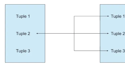
■ One-to-many relationship:฀A฀one-to-many฀relationship฀maps฀a฀single฀row฀in

table A to multiple other rows in table B. However, each row in table B maps to only a single฀row฀in฀table฀A฀(see฀Figure฀1.2).

■ Many-to-many relationship:฀A฀many-to-many฀relationship฀maps฀multiple฀rows

in table A to multiple rows in table B and maps multiple rows in table B to multiple

rows฀in฀table฀A฀(see฀Figure฀1.3).

Referential Integrity

When using relationships in the relational model, it is important to ensure that a foreign key in a referenced table can be resolved to a tuple in the referring table. This concept is known as referential integrity. Most relational database management systems help to enforce referential integrity so that tables don’t have foreign keys that cannot be resolved.

The concept of relationships is of great importance to the relational model as it allows

the฀attributes฀of฀a฀relation฀to฀be฀atomic.฀For฀example,฀let’s฀consider฀a฀conceptual฀data฀ Figure 1.2 One-to-many relationship

model that tracks mobile device information in addition to the os฀relation฀from฀Table฀1.1.฀

The฀relational฀schema฀for฀the฀database฀now฀looks฀like฀the฀following:

os(version, codename, api)

device(version, manufacturer, os_version, os_codename, os_api)

The device relation has attributes that define the characteristics of the hardware and the software. In addition, the os relation contains the characteristics of the OS software. If tuples฀are฀added,฀the฀tabular฀form฀of฀the฀relations฀would฀look฀like฀Table฀1.2.

While the relation looks innocent enough, it has duplicate attributes that do not fit into a normalized form of the relational model. Specifically, values for the os_version, os_codename, and os_api attributes are repeated in multiple tuples in the relation. In addition, the same values are part of the os฀relation฀from฀Table฀1.1.฀Now,฀imagine฀that฀an฀attribute฀of฀ the os relation needs to be updated. In addition to directly modifying the os relation, each tuple of the device relation that references the os information needs to be updated. Duplicate copies of the data require multiple update operations when the data changes.

To solve this issue and make relations conform to a normal form, we can replace the os_version, os_codename, and os_api attributes in the device relation with the primary key from the os relation. This allows tuples in the device relation to reference tuples in the os relation. As mentioned previously, the primary key is a candidate key that is selected as the primary key.

The os฀relation฀has฀two฀candidate฀keys:฀the฀version and the api฀attributes.฀Notice฀ that the codename attribute is not a candidate key as it does not uniquely identify a tuple in the relation (multiple tuples share the codename฀“Lollipop”).฀For฀this฀example,฀we฀use฀ version as the primary key for the os฀relation.฀Using฀version as the primary key for os, we can rewrite the device relation to use the os foreign key to add the normalized relationship to the device relation. The updated device฀relation฀now฀looks฀like฀Table฀1.3.

Table 1.2 device Relation

version manufacturer os_version os_codename os_api

Galaxy Nexus Samsung 4.3 Jelly Bean 18

Nexus 5 LG 5.1 Lollipop 21

Nexus 6 Motorola 5.1 Lollipop 21

Table 1.3 Normalized device Relation

version manufacturer os_version

Galaxy Nexus Samsung 4.3

Nexus 5 LG 5.1

With the updated structure, an update to the os relation is immediately reflected across the database since the duplicate attributes have been replaced by a reference to the os relation. Additionally, the device relation does not lose any os information since it can use the os_version attribute to look up attributes from the os relation.

Relational Languages

Thus far in the discussion of the relational model, we have focused on model structure. Tables, attributes, tuples, and domains provide a way to format the data so it fits the model, but we also need a way to both query and manipulate that model.

The two languages most used to manipulate a relational model are relational algebra

and relational calculus. While relational algebra and relational calculus seem different, it is important to remember that they are equivalent. Any expression that can be written in one can also be written in the other.

Relational calculus, and to some extent relational algebra, is the basis for

higher-level฀manipulation฀languages฀like฀SQL฀and฀SEQUEL.฀While฀a฀user฀does฀not฀directly฀use฀

relational algebra or relational calculus to work with a database (higher-level languages are used instead), it is important to have at least a basic understanding of them to better comprehend what the higher-level languages are doing.

Relational Algebra

Relational algebra is a language that describes how the database should run a query in order to return the desired results. Because relational algebra describes how to run a query, it is referred to as a procedural language.

A relational algebra expression consists of two relations that act as operands and an operation. The operation produces an additional relation as output without any side effects on the input operands. Relations are closed under relational algebra, meaning that both the inputs and the outputs of an expression are relations. The closure property allows expressions to be nested using the output of one expression to be the input of another.

All relational algebra operations can be broken down into a base set of five operations. While other operations do exist, any operation outside the base set can be expressed in terms of the base set of operations. The base set of operations in relational algebra consists of selection, projection, Cartesian product, union, and

set difference.

Relational algebra operations can operate on either a single relation (unary) or a pair of relations (binary). While most operations are binary, the selection and projection operations operate on a single relation and are unary.

In addition to the base operations, this section discusses the intersection and join

operations.

Union (A ∪ B)

The union operator produces a relation that includes all the tuples in the operand

relations฀(see฀Table฀1.6).฀It฀can฀be฀thought฀of฀as฀an฀“or”฀operation฀in฀that฀the฀output฀

relation has all the members that are in either relation A OR relation B.

Intersection (A ∩ B)

The intersection operator produces a relation that includes all tuples in both relation A and฀relation฀B฀(see฀Table฀1.7).

Table 1.4 Relation A Color

Red White Blue

Table 1.5 Relation B Color

Orange White Black

Table 1.6 A ∪ B Color

Red White Blue Orange Black

Table 1.7 A ∩ B Color

Difference (A - _B)

The difference operator produces a relation that contains the tuples that are members of

the฀left฀operand฀without฀the฀tuples฀that฀are฀members฀of฀the฀right฀operand฀(see฀Table฀1.8).

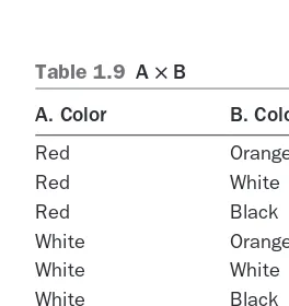
Cartesian Product (A ë _B)

The฀Cartesian฀product฀produces฀a฀relation฀that฀includes฀all฀possible฀ordered฀pairings฀of฀all฀ tuples฀from฀operand฀A฀with฀all฀tuples฀from฀operand฀B฀(see฀Table฀1.9).฀The฀degree฀of฀the฀

output relation is the sum of the degree of each operand relation. The cardinality of the output relation is the product of the cardinalities of the input relations. In our example,

both฀relations฀A฀and฀B฀have฀a฀degree฀of฀1.฀Therefore,฀the฀output฀relation฀has฀a฀degree฀ of฀1+฀1฀=฀2.฀Similarly,฀both฀relations฀A฀and฀B฀have฀a฀cardinality฀of฀three,฀so฀the฀output฀

relation฀has฀a฀degree฀of฀3฀∗฀3฀=฀9.

Selection (σ

predicate(A))

Selection produces a relation with only the tuples from the operand that satisfy a given predicate. Remember that, unlike the previous operations, selection is a unary operation and operates on only a single relation.

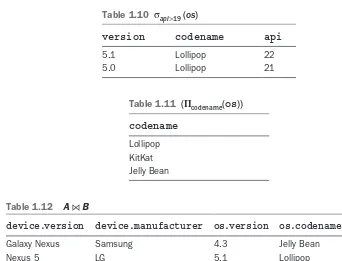
As an example of the selection operation, we again consider the os relation from earlier in the chapter. In the example, the os relation is being searched for all tuples that contain an api฀value฀that฀is฀greater฀than฀19฀(see฀Table฀1.10).

Table 1.8 A - B Color

Red Blue

Table 1.9 A ë _B

A. Color B. Color

Red Orange

Red White

Red Black

White Orange

White White

White Black

Blue Orange

Blue White

Projection (Π_{a1, a2,…,an}(A))

Projection produces a relation containing only the attributes that are specified on the operand. The output relation has the values from the attributes listed in the operand, and the operation removes the duplicates.

Like฀selection,฀projection฀is฀also฀a฀unary฀operation฀working฀on฀a฀single฀input฀relation.฀ As฀an฀example,฀we฀again฀use฀the฀relation฀depicted฀in฀Table฀1.1.฀This฀time,฀only฀the฀values฀

for the attribute codename฀are฀included฀in฀the฀resulting฀relation฀(see฀Table฀1.11).

Joins

The฀join฀relations฀can฀be฀considered฀a฀class฀of฀relations฀that฀are฀similar฀to฀the฀Cartesian฀ product฀of฀two฀operand฀relations.฀Usually,฀a฀query฀does฀not฀need฀to฀return฀the฀complete฀ pairing฀of฀tuples฀from฀the฀two฀operands฀that฀are฀produced฀by฀the฀Cartesian฀product.฀

Instead, it is usually more useful to limit the output relation to only those pairings that meet certain criteria. This is where the different join operations are useful.

Natural join is a useful join variant as it conceptually allows two relations to be combined into a single relation connecting the relations over a set of common attributes.

For฀example,฀if฀we฀consider฀the฀os฀relation฀in฀Table฀1.1฀and฀the฀normalized฀device

relation฀in฀Table฀1.3,฀we฀can฀produce฀a฀relation฀that฀combines฀the฀two฀relations฀using฀the฀

device.os_version and os.version attributes from each of the input relations. The

results฀are฀depicted฀in฀Table฀1.12. Table 1.10 σ

api>19 (os)

version codename api

5.1 Lollipop 22

5.0 Lollipop 21

Table 1.11 (Π

codename(os))

codename

Lollipop KitKat Jelly Bean

Table 1.12 A⋈ B

device.version device.manufacturer os.version os.codename os.api

Galaxy Nexus Samsung 4.3 Jelly Bean 18

Nexus 5 LG 5.1 Lollipop 21

Notice฀how฀the฀result฀of฀the฀natural฀join฀is฀the฀same฀unnormalized฀relation฀as฀in฀

Table 1.2.฀By฀using฀a฀join฀operation,฀we฀are฀now฀able฀to฀perform฀additional฀operations฀on฀ the output relation to produce the same results that would have been obtained if the data was combined in one table.

Natural฀join฀is฀really฀a฀specific฀type฀of฀theta join that uses the equality operation over a set of attributes. Theta join allows the use of any operation to combine the two operand relations. Equality (producing a natural join) is just one of the most common cases.

Relational Calculus

Relational calculus is another relational language that can be used to query and modify a

relational฀model.฀Codd฀made฀the฀proposal฀for฀tuple฀relational฀calculus฀after฀his฀paper฀that฀

introduced the relational model.

As discussed previously, relational algebra describes how data should be retrieved. Using฀ relational calculus, we can describe what needs to be retrieved and leave the details of how the data is retrieved to the database. Because relational calculus is concerned with describing what to retrieve, it can be classified as a declarative language.

There฀are฀two฀forms฀of฀relational฀calculus:฀tuple relational calculus and domain relational calculus. Both forms are described in the following sections.

Tuple Relational Calculus

In tuple relational calculus, the tuples of a relation are evaluated against a predicate. The output of an expression is the relation that contains the tuples that make the predicate true. Again, with relational calculus, we only need to specify what we want and let the system determine the best way to fulfill the request.

If we again consider the os฀relation฀listed฀in฀Table฀1.1,฀we฀can฀formulate฀a฀tuple฀

relational฀calculus฀query฀in฀words.฀It฀would฀read฀something฀like฀this:

Return all tuples from the relation os where the codename฀is฀“Lollipop.”

Notice฀that฀this฀is฀the฀same฀query฀that฀we,฀in฀the฀previous฀section,฀defined฀using฀

relational algebra. While the text representation is generally how humans think about tuple relational calculus, we often use a shorthand notation to define the relation. The shorthand notation for this query would be

{x|os(x) ∧x.codename= ‘Lollipop’}

This query would return all attributes for tuples that satisfy the predicate. We can also limit the attributes that are returned by the query. A query that would return only the codename฀when฀it฀is฀equal฀to฀“Lollipop”฀would฀look฀like฀this:

{x.codename|os(x) ∧x.codename฀=฀‘Lollipop’}

Domain Relational Calculus

Database Languages

While the structure of a relational database is important, it is also necessary to be able

to฀manipulate฀the฀data฀that฀is฀housed฀in฀the฀database.฀In฀his฀1970฀paper,฀Codd฀started฀ describing฀a฀sub-language฀called฀ALPHA฀based฀on฀predicate฀calculus฀declaring฀relations,฀

their attributes, and their domains.

ALPHA

While฀the฀ALPHA฀language฀was฀never฀developed,฀it฀did฀lay฀the฀foundation฀for฀modern-day languages used by most relational database systems toWhile฀the฀ALPHA฀language฀was฀never฀developed,฀it฀did฀lay฀the฀foundation฀for฀modern-day. It is important to point out

that฀it฀was฀not฀Codd’s฀intent฀to฀provide฀a฀full฀implementation฀of฀such฀a฀language฀in฀a฀

paper that introduced the relational model. Instead, he presented some of the concepts and features that such a language would include. In addition, he described the language’s relationship with a higher-level language as a “proof of concept” about what the language could do with a relational model.

The฀features฀of฀ALPHA฀that฀Codd฀described฀included฀the฀retrieval,฀modification,฀

insertion, and deletion of data.

In฀addition฀to฀describing฀what฀the฀language฀could฀do,฀Codd฀went฀into฀the฀details฀of฀

what the language should not do. Since the main objective of the language is to interact with a relational data model, the semantics of the language specify what data to retrieve as opposed to how to retrieve it. This is an important detail and is a language feature that has

been฀carried฀through฀to฀modern-day฀SQL.

ALPHA฀was฀described฀as฀a฀“sub-language”฀that฀would฀exist฀along฀with฀another฀ higher-level฀“host”฀language.฀This฀implies฀that฀ALPHA฀was฀never฀meant฀to฀be฀a฀complete฀ language฀on฀its฀own.฀For฀example,฀features฀like฀arithmetic฀functions฀would฀be฀intention

-ally฀left฀out฀of฀ALPHA฀as฀they฀would฀be฀implemented฀in฀the฀host฀language฀and฀called฀ from฀ALPHA.

QUEL

QUEL฀was฀a฀database฀language฀developed฀at฀UC฀Berkeley฀based฀on฀Codd’s฀ALPHA฀ language.฀It฀was฀shipped฀as฀part฀of฀the฀Ingres฀DBMS฀and฀has฀roots฀in฀POSTQUEL฀which฀ was฀shipped฀with฀early฀versions฀of฀the฀Postgres฀database.฀QUEL฀was฀included฀as฀part฀of฀ early฀relational฀databases฀but฀has฀more฀recently฀been฀supplanted฀by฀SQL฀in฀most฀modern฀

relational database systems.

SEQUEL

Structured฀English฀QUEry฀Language฀(SEQUEL)฀was฀the฀name฀given฀to฀SQL฀when฀it฀

was originally developed by IBM. However, due to trademark infringements, the name

was฀shortened฀to฀Structured฀Query฀Language฀(SQL).฀SEQUEL฀was฀the฀first฀commercial฀ language฀to฀be฀implemented฀based฀on฀Codd’s฀ALPHA฀language.

As฀discussed฀earlier฀in฀the฀chapter,฀SQLite฀is฀the฀database฀system฀included฀as฀part฀

of Android. In addition to implementing a way to store relational data, it includes an

Summary

Relational databases offer a powerful mechanism to both store and operate on data. The introduction฀of฀the฀relational฀model฀by฀Edgar฀Codd฀in฀1970฀allowed฀database฀ technology to overcome many of the limitations that existed in earlier file-based models.

The relational model, along with relational algebra and relational calculus, allows a database to be queried and perform operations on the data it stores. By including the

concepts฀that฀define฀the฀relational฀languages฀in฀higher-level฀languages฀such฀as฀QUEL,฀ SEQUEL,฀and฀SQL,฀developers฀are฀able฀to฀harness฀the฀power฀of฀a฀relational฀database฀to฀

help support their software.

2

An Introduction to SQL

S

tructured฀Query฀Language฀(SQL)฀is฀one฀programming฀language฀used฀to฀interact฀with a฀relational฀database,฀and฀it฀is฀the฀language฀used฀in฀SQLite.฀The฀language฀supports฀the฀

ability to define database structure, manipulate data, and read the data contained in the database.

Although฀SQL฀has฀been฀standardized฀by฀both฀the฀American฀National฀Standards฀ Institute฀(ANSI)฀and฀the฀International฀Organization฀for฀Standardization฀(ISO),฀vendors฀

frequently add proprietary extensions to the language to better support their platforms.

This฀chapter฀primarily฀focuses฀on฀SQL฀as฀it฀is฀implemented฀in฀SQLite,฀the฀database฀ system฀that฀is฀included฀in฀Android.฀Most฀of฀the฀concepts฀in฀this฀chapter฀do฀apply฀to฀SQL฀

in general, but the syntax may not be the same for other database systems.

This฀chapter฀covers฀three฀areas฀of฀SQL:

■ Data฀Definition฀Language฀(DDL) ■ Data฀Manipulation฀Language฀(DML) ■ Queries

Each area has a different role in a database management system (DBMS) and a different subset of commands and language features.

Data Definition Language

Data฀Definition฀Language฀(DDL)฀is฀used฀to฀define฀the฀structure฀of฀a฀database.฀This฀

includes the creation, modification, and removal of database objects such as tables, views,

triggers,฀and฀indexes.฀The฀entire฀collection฀of฀DDL฀statements฀defines฀the฀schema for the database. The schema is what defines the structural representation of the database. The following฀SQL฀commands฀are฀usually฀used฀to฀build฀DDL฀statements:

■ CREATE:฀Creates฀a฀new฀database฀object ■ _ALTER:฀Modifies฀an฀existing฀database฀object ■ DROP:฀Removes฀a฀database฀object

Tables

Tables,฀as฀discussed฀in฀Chapter฀1,฀“Relational฀Databases,”฀provide฀the฀relations฀in฀a฀

relational database. They are what house the data in the database by providing rows

representing฀a฀data฀item,฀and฀columns฀representing฀attributes฀of฀each฀item.฀Table฀2.1฀shows฀

an example of a table that contains device information.

SQLite฀supports฀the฀CREATE, ALTER, and DROP commands with regard to tables. These commands allow tables to be created, mutated, and deleted respectively.

CREATE TABLE

The CREATE TABLE statement begins by declaring the name of the table that will be created฀in฀the฀database,฀as฀shown฀in฀Figure฀2.1.฀Next,฀the฀statement฀defines฀the฀ columns of the table by providing a column name, data type, and any constraints

for฀the฀column.฀Constraints฀place฀limits฀on฀the฀values฀that฀can฀be฀stored฀in฀a฀given฀

attribute of a table.

Table 2.1 Device Table

model nickname display_size_inches

Nexus One Passion 3.7

Nexus S Crespo 4.0

Galaxy Nexus Toro 4.65

Nexus 4 Mako 4.7

CREATE

TEMP

TABLE TEMPORARY

schema-name . table-name

select-stmt AS

EXISTS

column-def ,

) (

WITHOUT ROWID NOT

IF

table-constraint ,

Figure 2.1 Overview of the CREATE TABLE statement

Listing฀2.1฀shows฀a฀CREATE TABLE statement that creates a table named device with

three฀columns:฀model, nickname, and display_size_inches.

Listing 2.1 Creating the device Table CREATE TABLE device (model TEXT NOT NULL,

nickname TEXT,

display_size_inches REAL);

Note

The discussion of SQL data types is deferred to Chapter 3, “An Introduction to SQLite.” For now, it is enough to know that TEXT represents a text string and REAL a floating-point number.

If฀the฀SQL฀statement฀from฀Listing฀2.1฀is฀run฀and฀returns฀without฀an฀error,฀the฀device

table฀is฀created฀with฀three฀columns:฀model, nickname, and display_size_inches of types TEXT, TEXT, and REAL respectively. In addition, the table has a constraint on the model column to ensure that every row has a non-null model name. The constraint is created by appending NOT NULL to the end of the column name in the CREATE statement. The NOT NULL฀constraint฀causes฀SQLite฀to฀throw฀an฀error฀if฀there฀is฀an฀attempt฀to฀insert฀ a row into the table that contains a null value for the model column.

At this point, the table can be used to store and retrieve data. However, as time passes, it is often necessary to make changes to existing tables to support the changing needs of software. This is done with an ALTER TABLE statement.

ALTER TABLE

The ALTER TABLE statement can be used to modify an existing table by either adding new columns or renaming the table. However, the ALTER TABLE statement does have

limitations฀in฀SQLite.฀Notice฀from฀Figure฀2.2฀that฀there฀is฀no฀way฀to฀rename฀or฀remove฀

a column from a table. This means that once a column is added, it will always be a part of the table. The only way to remove a column is to remove the entire table and re-create

ALTER TABLE schema-name . table-name

new-table-name column-def RENAME TO

COLUMN ADD

Figure 2.2 Overview of the ALTER TABLE statement

the table without the column to be removed. Doing this, however, also removes all the data that was in the table. If the data is needed when the table is re-created, an app must manually copy the data from the old table into the new table.

As฀an฀example,฀the฀SQL฀code฀to฀add฀a฀new฀column฀to฀the฀device table is shown in

Listing฀2.2.฀The฀new฀column฀is฀named฀memory_mb and it is of type REAL. It is used to track the amount of memory in a device.

Listing 2.2 Adding a New Row to the device Table ALTER TABLE device ADD COLUMN memory_mb REAL;

DROP TABLE

The DROP TABLE statement is the simplest table operation; it removes the table from the

database฀along฀with฀all฀the฀data฀it฀contains.฀Figure฀2.3฀shows฀an฀overview฀of฀the฀DROP TABLE statement. In order to remove a table, the DROP TABLE statement needs only the name of the table to be removed.

The device฀table฀can฀be฀removed฀with฀the฀statement฀shown฀in฀Listing฀2.3.

Listing 2.3 Removing the device Table DROP TABLE device;

Care฀should฀be฀taken฀when฀using฀the฀DROP TABLE statement. Once the DROP TABLE statement completes, the data is irrevocably removed from the database.

Indexes

An index is a database object that can be used to speed up queries. To understand what an

index฀is,฀a฀discussion฀of฀how฀databases฀(SQLite฀in฀this฀case)฀find฀rows฀in฀a฀table฀is฀helpful.

Suppose an app needs to find a device with a specific model from the device table

shown฀in฀Table฀2.1.฀The฀application฀code฀would฀run฀a฀query฀against฀the฀table,฀passing฀the฀ desired฀model฀name.฀Without฀an฀index,฀SQLite฀would฀then฀have฀to฀examine฀every฀row฀

in the table to find all rows that match the model name. This is referred to as a full table scan as the entire table is being read. As the table grows, a full table scan takes more time as the database needs to inspect an increasing number of rows. It would take significantly more time to perform a full table scan on a table with four million rows than on a table with only four rows.

schema-name . table-name TABLE IF EXISTS

DROP

Figure 2.3 Overview of the DROP TABLE statement

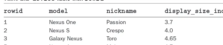
An index can speed up a query by keeping track of column values in an additional table that can be quickly scanned to avoid a full table scan. Table 2.2 shows another version of the device฀table฀presented฀in฀Table฀2.1.

Notice฀the฀new฀column฀in฀Table฀2.2฀called฀rowid.฀SQLite฀automatically฀creates฀this฀ column when creating a table unless you specifically direct it not to. While an app will logically consider the device฀table฀to฀look฀like฀Table฀2.1฀(without฀the฀rowid), in memory the device table actually looks more like Table 2.2 with the rowid included.

Note

The rowid column can also be accessed using standard SQL queries.

The rowid฀is฀a฀special฀column฀in฀SQLite฀and฀can฀be฀used฀to฀implement฀indexes.฀ The rowid for each row in a table is guaranteed to be an increasing integer that uniquely identifies the row. However, notice in Table 2.2 that the rowid values may not be consecutive. This is because rowids are generated as rows are inserted to a table, and rowid values are not reused when rows are removed from a table. In Table 2.2, a row with a rowid฀of฀4฀was฀inserted฀into฀the฀table฀at฀one฀point฀but฀has฀since฀been฀deleted.฀ Even though rowids may not be consecutive, they remain ordered as rows are added to the table.

Using฀the฀rowid,฀SQLite฀can฀quickly฀perform฀a฀lookup฀on฀a฀row฀since฀internally฀it฀ uses a B-tree to store row data with the rowid as the key.

Note

Using the rowid to query a table also prevents the full table scan. However, rowids are usually not convenient to use as they rarely have any other purpose in an app’s business logic.

When฀an฀index฀is฀created฀for฀a฀table฀column,฀SQLite฀creates฀a฀mapping฀of฀the฀row฀

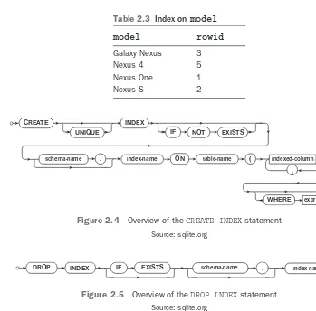
values for that column and the corresponding rowid.฀Table฀2.3฀shows฀such฀a฀mapping฀for฀ the model column of the device table.

Notice฀that฀the฀model฀names฀are฀sorted.฀This฀allows฀SQLite฀to฀perform฀a฀binary฀search฀ to฀find฀the฀matching฀model.฀Once฀it฀is฀found,฀SQLite฀can฀access฀the฀rowid for the model and use that to perform the lookup of the row data in the device table without the need for a full table scan.

Table 2.2 device Table with rowid

rowid model nickname display_size_inches

1 Nexus One Passion 3.7

2 Nexus S Crespo 4.0

3 Galaxy Nexus Toro 4.65

CREATE

UNIQUE

INDEX

IF NOT EXISTS

schema-name . index-name ON table-name (

,

)

indexed-column expr

WHERE

Figure 2.4 Overview of the CREATE INDEX statement

Source: sqlite.org

INDEX

DROP IF EXISTS schema-name . index-name

Figure 2.5 Overview of the DROP INDEX statement

Source: sqlite.org

Table 2.3 Index on model

model rowid

Galaxy Nexus 3

Nexus 4 5

Nexus One 1

Nexus S 2

CREATE INDEX

The CREATE INDEX statement needs a name as well as a column definition for the index. In the simplest case, the index has a column definition that includes a single column that

is฀frequently฀used฀to฀search฀a฀table฀during฀queries.฀Figure฀2.4฀shows฀the฀structure฀of฀the฀

CREATE INDEX statement.

Listing฀2.4฀shows฀how฀to฀create฀an฀index฀on฀the฀model column of the device table.

Listing 2.4 Creating an Index on model

CREATE INDEX idx_device_model ON device(model);

Unlike฀tables,฀indexes฀cannot฀be฀modified฀once฀they฀are฀created.฀Therefore,฀the฀ALTER keyword cannot be applied to indexes. To modify an index, the index must be deleted with a DROP INDEX statement and then re-created with a CREATE INDEX statement.

DROP INDEX

Listing฀2.5฀shows฀how฀to฀drop฀the฀index฀that฀was฀created฀in฀Listing฀2.4.

Listing 2.5 Deleting the Index on model

DROP INDEX idx_device_model;

Views

A view can be thought of as a virtual฀table฀in฀a฀database.฀Like฀a฀table,฀it฀can฀be฀queried฀ against to get a result set. However, it does not physically exist in the database in the same way that a table does. Instead, it is the stored result of a query that is run to generate the

view.฀Table฀2.4฀shows฀an฀example฀of฀a฀view.

Notice฀that฀the฀view฀from฀Table฀2.4฀contains฀only฀a฀subset฀of฀the฀columns฀of฀the฀

device table. Even if more columns are added to the table, the view will remain the same.

Note

SQLite supports only read-only views. This means that views can be queried but do not support the DELETE, INSERT, or UPDATE operations.

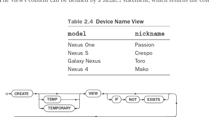
CREATE VIEW

The CREATE VIEW statement assigns a name to a view in a similar manner to other CREATE statements (CREATE TABLE, CREATE VIEW,฀etc.),฀as฀shown฀in฀Figure฀2.6.฀In฀addition฀to฀ a name, the CREATE VIEW statement includes a way to define the content of the view. The view’s content can be defined by a SELECT statement, which returns the columns

Table 2.4 Device Name View

model nickname

Nexus One Passion

Nexus S Crespo

Galaxy Nexus Toro

Nexus 4 Mako

CREATE

TEMP

VIEW

IF NOT EXISTS TEMPORARY

. (

,

)

AS select-stmt column-name

view-name schema-name

Figure 2.6 Overview of the CREATE VIEW statement

to be included in the view as well as places limits on which rows should be included in the view.

Listing฀2.6฀shows฀the฀SQL฀code฀needed฀to฀create฀the฀view฀from฀Table฀2.4.฀The฀code฀

creates a view named device_name which includes the model and nickname columns from the device table. Because the SELECT statement has no WHERE clause, all rows from the device table are included in the view.

Listing 2.6 Creating the device_name View

CREATE VIEW device_name AS SELECT model, nickname FROM device;

Note

SELECT statements are covered in more detail later in the chapter.

Views฀in฀SQLite฀are฀read-only฀and฀don’t฀support฀the฀DELETE, INSERT, or UPDATE operations. In addition, they cannot be modified with an ALTER statement. As with indexes, in order to modify a view, it must be deleted and re-created.

DROP VIEW

DROP VIEW works like the other DROP commands that have been discussed thus far. It takes the name of the view to be deleted and removes it. The details of the DROP VIEW

statement฀can฀be฀seen฀in฀Figure฀2.7.฀

Listing฀2.7฀removes฀the฀device_name฀view฀that฀was฀created฀in฀Listing฀2.6.

Listing 2.7 Removing the device_name View DROP VIEW device_name;

Triggers

The฀final฀database฀object฀that฀can฀be฀manipulated฀by฀DDL฀is฀a฀trigger.฀Triggers฀provide฀a฀ way฀to฀perform฀an฀operation฀in฀response฀to฀a฀database฀event.฀For฀example,฀a฀trigger฀can฀be฀ created฀to฀run฀an฀SQL฀statement฀whenever฀a฀row฀is฀added฀or฀deleted฀in฀the฀database.

CREATE TRIGGER

Like฀other฀CREATE statements discussed previously, the CREATE TRIGGER statement assigns a name to a trigger by providing the name to the CREATE TRIGGER statement.

DROP VIEW IF EXISTS schema-name . view-name

Figure 2.7 Overview of the DROP VIEW statement

After the name, an indication of when the trigger needs to run is defined. This

definition฀of฀when฀a฀trigger฀should฀run฀has฀two฀parts:฀the฀operation฀that฀causes฀the฀ trigger฀to฀run,฀and฀when฀the฀trigger฀should฀run฀in฀relation฀to฀that฀operation.฀For฀

example, a trigger can be declared to run before, after, or instead of any DELETE, INSERT, or UPDATE operation. The DELETE, INSERT, and UPDATE operations are part of

SQL’s฀DML,฀discussed฀later฀in฀the฀chapter.฀Figure฀2.8฀shows฀an฀overview฀of฀the฀CREATE TRIGGER statement.

Listing฀2.8฀shows฀the฀creation฀of฀a฀trigger฀on฀the฀device table that sets the insertion time of any newly inserted rows.

TEMP TEMPORARY

CREATE TRIGGER

IF NOT

BEFORE AFTER

INSTEAD OF

ON table-name

column-name OF

DELETE INSERT

UPDATE

ROW WHEN expr

END

select-stmt delete-stmt insert-stmt

update-stmt ; ,

BEGIN

EACH FOR

trigger-name schema-name .

EXISTS

Figure 2.8 Overview of the CREATE TRIGGER statement

Listing 2.8 Creating a Trigger on the device Table ALTER TABLE device ADD COLUMN insert_date INTEGER;

CREATE TRIGGER insert_date AFTER INSERT ON device

BEGIN

UPDATE device

SET insert_date = datetime('now');

WHERE _ROWID_ = NEW._ROWID_;

END;

Before the insertion date can be tracked, the insert_date column must be added to the device table. This is done with an ALTER TABLE statement prior to the trigger being created (the insert_date column needs to exist before it can be referenced in the trigger definition).

After the ALTER TABLE statement has been run, the device table will contain the

values฀shown฀in฀Table฀2.5.

Notice฀that฀the฀value฀of฀insert_date is null for all rows. This is because the column was added after the table was created and the ALTER TABLE statement did not specify a default value to add to existing rows.

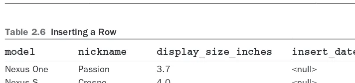
Now฀that฀the฀trigger฀is฀defined,฀the฀following฀INSERT statement can be run to insert a

new฀row฀in฀the฀table:

INSERT INTO device (model, nickname, display_size_inches)

VALUES ("new_model", "new_nickname", 4);

Table฀2.6฀shows฀the฀rows฀that฀are฀now฀in฀the฀device table.

Table 2.6 Inserting a Row

model nickname display_size_inches insert_date

Nexus One Passion 3.7 <null>

Nexus S Crespo 4.0 <null>

Galaxy Nexus Toro 4.65 <null>

Nexus 4 Mako 4.7 <null>

new_model new_nickname 4 2015-07-13 04:52:20

Table 2.5 Adding insert_date

model nickname display_size_inches insert_date

Nexus One Passion 3.7 <null>

Nexus S Crespo 4.0 <null>

Galaxy Nexus Toro 4.65 <null>