Development of a 1-km landcover dataset of China
using AVHRR data
Xiuwan Chen
a,), Ryutaro Tateishi
b, Changyao Wang
ca
Institute of Remote Sensing and GIS, Peking UniÕersity, Beijing 100871, China
b ( )
Center for EnÕironmental Remote Sensing CEReS , Chiba UniÕersity, 1-33 Yayoi-cho Inage-ku, Chiba 263, Japan
c
Institute of Remote Sensing Applications, Chinese Academy of Sciences, Beijing 100101, China
Received 28 June 1998; accepted 24 July 1999
Abstract
This paper describes the development of a 1-km landcover dataset of China by using monthly NDVI data spanning April 1992 through March 1993. The method used combined unsupervised and supervised classification of NDVI data from
Ž .
AVHRR. It is composed of five steps: a unsupervised clustering of monthly AVHRR NDVI maximum value composites is Ž .
performed using the ISOCLASS algorithm; b preliminary identification is carried out with the addition of digital elevation models, eco-region data and a collection of other landcoverrvegetation reference data to identify the clusters with single
Ž .
landcover classes; c re-clustering is performed of clusters with size greater than a given threshold value and containing two Ž .
or more disparate landcover classes; d cluster combining is performed to combine all clusters with a single landcover class Ž .
in one cluster, and all other clusters into one mixed cluster; and e supervised classification is used to carry out post-classification of the mixed cluster generated in the previous step by using the maximum likelihood algorithm and the identified single landcover classes of the previous step as training data. The classification is based on extensive use of computer-assisted image processing and tools, as well as the skills of the human interpreter to take the final decisions regarding the relationship between spectral classes defined using unsupervised methods and landscape characteristics that are used to define landcover classes.q1999 Elsevier Science B.V. All rights reserved.
Ž .
Keywords: landcover; dataset; China; AVHRR; Normalised Difference Vegetation Index NDVI
1. Introduction
Landcoverrlanduse is one of the main factors that have a great impact on the natural environment and the social and economic activities of human beings. Multi-temporal, multi-resolution landcoverruse
Ž
datasets at different scales local, regional, national,
)Corresponding author. Fax: q86-10-6851-3212; E-mail: [email protected], [email protected]
.
continental, global, etc. are very useful for scientific research in various disciplines and management of natural resources and environment. China is a devel-oping country with complex terrestrial landcover. Thus, it is necessary to pay enough attention to landcover monitoring and landuse planning, so as to protect natural environment and ecosystem effec-tively. Many programs have been initiated andror finished to extract landcoverrlanduse information
Ž .
for small important areas e.g., urban areas at local
0924-2716r99r$ - see front matterq1999 Elsevier Science B.V. All rights reserved. Ž .
or regional scale by using high-resolution satellite Ž . data such as Landsat Thematic Mapper TM , SPOT etc. But there is little research involving large areas, like the whole of China, by using coarse-resolution Že.g., 1 km satellite data..
The National Oceanic and Atmospheric
Adminis-Ž .
tration NOAA Advanced Very High Resolution
Ž .
Radiometer AVHRR sensor has been in operation since 1982 and collects daily coverage of the earth at a nominal 1 km pixel resolution. AVHRR data and
Ž .
the Normalized Difference Vegetation Index NDVI calculations and other interpretations derived from them are very important for monitoring regional, continental and global landcover conditions.
Efforts have been made by many scientists all over the world to map landcover using AVHRR and NDVI. For example, the International Geosphere-Biosphere Programme-Data and Information System ŽIGBP-DIS began the 1 km landcover project in. 1990 and a global 1 km landcover dataset was created on a continent-by-continent basis. The classi-fication approach used is based on unsupervised classification of NDVI time series with ancillary
Ž
datasets, such as digital elevation models Loveland .
et al., 1991; Brown et al., 1993 . Related activities have also been initiated in Asian and Oceanic coun-tries. The Asian Association on Remote Sensing ŽAARS established the Working Group on 1 km. Landcover Database of Asia in October 1993. The Working Group consists of 44 members from 27 Asian and Oceanic countries, and aims to produce a landcover dataset of Asia and Oceania using 1 km AVHRR data. The development of a 1 km landcover dataset for the whole of China is an important objec-tive of the Working Group.
2. Data acquisition and processing
The satellite data used in this study are the 10-day composite NDVI datasets produced by the Global Land 1 km AVHRR Dataset Program at USGS EROS Data Center. The data were collected between April 1992 and March 1993. Monthly values were derived from the 10-day composites. The use of monthly values rather than 10-day composite values represents a compromise between temporal
fre-Ž
quency and the need for cloud-free data Moody and .
Strahler, 1994 . It also provides a means to reduce data volume, while maintaining annual phenological information. The recomposing of the NDVI data was performed for the whole of Asia from top-left at the
Ž .
Barents Sea 908N, 258E to down-right at the Coral
Ž . China, except some islands.
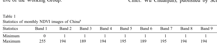
After screening the 12 monthly NDVI images, the data for November 1992 and March 1993 were discarded from the analysis. Thus, 10 monthly datasets including that from April 1992 to October 1992 and from December 1992 to February 1993 were used to carry out the landcover classification of China. Statistics for the data used in the study area are shown in Table 1. The data are shown with values in the range of 0 to 255, transformed from the original data with values in the range of y1 to 1.
Available conventional data and maps for this Ž .
study include: a Landuse map of China Ž1:1,000,000 , edited by the Editorial Committee for.
Ž
the 1:1,000,000 Landuse Map of China Editor-in-.
Chief: Wu Chuanjun , published by Science Press,
Table 1
Statistics of monthly NDVI images of Chinaa
Statistics Band 1 Band 2 Band 3 Band 4 Band 5 Band 6 Band 7 Band 8 Band 9 Band 10
Minimum 0 1 1 1 1 1 1 1 1 1
Maximum 255 194 189 194 195 189 195 194 194 192
Mean 151 99 100 103 108 113 113 114 109 105
Median 175 116 116 121 122 129 128 136 128 122
Std. Dev. 77.2 49.7 50.0 49.3 53.0 55.8 58.3 58.2 54.9 53.4
Corr. Eigenval. 9.581 0.219 0.091 0.027 0.024 0.017 0.014 0.010 0.010 0.006
Cov. Eigenval. 30593.0 724.8 279.4 87.8 75.5 51.4 46.4 31.7 28.6 15.6
a
Ž .
Beijing, 1990; b Resources and environment data
Ž .
of China 1:4,000,000 , produced by the State Key Laboratory of Resources and Environment Informa-tion Systems of the Institute of Geography, at the
Ž
Chinese Academy of Sciences, Beijing November .
1996 . The data include 17 specific datasets: national boundaries, provincial boundaries, county bound-aries, canals, desertification, geomorphology, glaciers, landslide development, railway system, rivers, main road system, soils, wetlands,
topogra-Ž .
phy, vegetation, and surface waters; c GTOPO30: Global 30 ArcSecond Elevation Dataset that USGS Ž . offers to the public through the Internet; and d Ground truth data acquired by the AARS Global 4-min Landcover Dataset Program.
The image analysis and classification, and geo-graphic information processing were carried out us-ing the ER Mapper andCITYSTARsoftware tools. ER Mapper is a geographic image processing software produced by the Earth Resources Mapping Pty. Ltd., which can display and enhance raster data, display and edit vector data, and link them with data from geographic and land information systems, database management systems or virtually any other sources ŽEarth Resources Mapping Pty. Ltd., 1995 .. CITYS -TAR is an integrated RS, GIS and GPS multimedia system, developed by the Institute of Remote Sens-ing and GIS, PekSens-ing University.
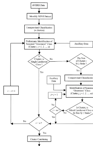
3. Methodology of landcover classification
The method used in this study combines unsuper-vised classification and superunsuper-vised classification of
Ž .
NDVI data Chen, 1998 . It is composed of five steps as shown in Fig. 1. The LCWGrAARS Land-cover Classification System was used to develop the
Ž
landcover classification in China Tateishi and Wen, .
1996 . The classification is based on the use of computer-assisted image processing and tools, as well as the skills of the human interpreter to take the final decisions regarding the relationship between
Ž
spectral classes defined using unsupervised meth-.
ods and landscape characteristics that are used to define landcover classes.
3.1. UnsuperÕised classification
The initial segmentation of the 10-month NDVI composites into seasonal greenness classes is
per-formed using unsupervised clustering. This classifi-cation method is preferred for studies in which the location and characteristics of specific classes are unknown. Unsupervised classification uses clustering to identify natural groupings of pixels with similar NDVI properties. In this case, the clusters corre-spond to annual sequences of green-up, peak, and senescence. Clustering algorithms used for the unsu-pervised classification of remotely sensed data gen-erally vary according to the efficiency with which the clustering takes place. Different criteria of
effi-Ž
ciency lead to different approaches Haralick and Fu, .
1983 . The specific clustering algorithm used isISO -Ž
CLASS ER Mapper, Earth Resources Mapping Pty.
.
Ltd., 1995 . It calculates class means that are evenly distributed in the data space and then iteratively clusters the remaining pixels using minimum dis-tance techniques. Each iteration recalculates means and reclassifies pixels with respect to the new means. This process continues until the number of pixels in each class changes by less than the selected pixel change threshold or the maximum number of itera-tions is reached.
3.2. Preliminary identification of greenness clusters
The purpose of this step is to provide a general understanding of the characteristics of each cluster Žor seasonal greenness class and to determine which. clusters include a single landcover class within their spatial distribution. Clusters with a single landcover class may be also used as training data for the final supervised classification. Preliminary identification involves inspecting the spatial patterns and spectral or multitemporal statistics of each class, comparing each class to reference data, and taking decisions concerning landcover types. This step includes two primary tasks. One is the generation of statistics and graphics for each of the n clusters, describing their relationship to the available ancillary data. The other is the interpretation of the summaries, graphs, and reference data to determine the general landcover class or classes associated with each seasonal green-ness cluster and to identify the clusters that represent single landcover classes.
3.3. Reprocessing of mixed classes
Fig. 1. Flowchart of landcover dataset development.
For the clusters with two or more landcover classes, a threshold value of the cluster size, Smin, is used to
Ž . equal to or greater than Smin i.e., SiGSmin , then this cluster should be re-clustered by the unsuper-vised algorithm.
The Smin value is determined subjectively based mainly on actual conditions. For example, it can be 1% or 5% of the total size of all clusters.
Generally, this is an iterative process in which the initial criteria are tested, refined, and finally used to permanently modify the original class. This results in a number of new seasonal greenness classes, that through the following steps, become the final land-cover classes.
3.4. Cluster combining
The cluster combining is performed to combine those clusters with the same landcover class, and combine all other clusters with Si-Smin into one mixed cluster. The former are directly used in the final landcover regions, while the latter are re-classi-fied in next step.
3.5. SuperÕised classification
A maximum likelihood algorithm was chosen to perform the supervised classification, due to its
suc-Ž
cessful use in prior research Chen, 1997; Chen and .
Hu, 1999 .
The maximum likelihood decision rule assigns each pixel having pattern measurements or features
X to the class c, whose units are most probable or
likely to have given rise to the feature vector X ŽSwain and Davis, 1978; Foody et al., 1992 . It. assumes that the training data statistics for each class in each band are normally distributed, i.e., Gaussian ŽBlaisdell, 1993 . In other words, training data with. bi- or tri-modal histograms in a single band are not ideal. The decision rule applied to the unknown
Ž
measurement vector X is Swain and Davis, 1978; .
with M the mean vector and det Vc c the determi-nant of the covariance matrix V . Therefore, to clas-c
sify the measurement vector X of an unknown pixel into a class, the maximum likelihood decision rule computes the value p for each class. Then, it as-c
signs the pixel to the class that has the maximum value.
This assumes that each class has an equal proba-bility of occurring in the terrain. However, in most remote sensing applications, there is a high probabil-ity of encountering some classes more often than others. Thus, we would expect more pixels to be classified as some class simply because it is more prevalent in the terrain. It is possible to include this
Ž .
valuable a priori information prior knowledge in the classification decision. We can do this by weight-ing each class c by its appropriate a priori probabil-ity, a . The equation then becomes:c
Decide X is in class c if, and only if,
This algorithm was used to carry out post-classifi-cation of the mixed cluster generated in the previous step. The classes with single landcover classes, iden-tified and combined in previous steps, are used as training data.
Following the generation of the landcover classifi-cation in this step, the remaining steps in the dataset generation are as follows.
Ž .1 Generate final attributes of the landcover dataset and sort out relative data such as landcover classification system, file listing, ground truth data, and any additional sources used in dataset production andror useful for reference.
Ž .2 Produce landcover map with legend and ad-ministrative boundaries.
4. Results and discussion
4.1. LandcoÕer classification system
Certain classification schemes have been devel-oped that can readily incorporate landuse andror landcover data obtained by interpreting remotely sensed data, e.g., US Geological Survey Landuser Landcover Classification System, US Fish and Wildlife Service Wetland Classification System, NOAA CoastWatch Landcover Classification
Sys-Ž .
tem Jensen, 1996 and the LCWGrAARS Land-Ž
cover Classification System Tateishi and Wen, .
1996 . The LCWGrAARS Landcover Classification
Ž .
System was used in this study see Appendix A .
4.2. LandcoÕer classification
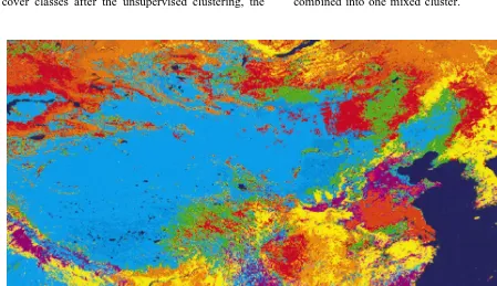
The ISOCLASS algorithm was used to perform
un-supervised clustering with 10-month composites AVHRR NDVI data for April 1992 through
Febru-Ž .
ary 1993 except November 1992 . In order to ensure that there will be enough clusters with single land-cover classes after the unsupervised clustering, the
maximum number of clusters which is an input parameter of this algorithm must be set high. In this case, it was selected as 100.
Ž .
Based on the clustering result Fig. 2 , statistics Žthe size of each clusters, mean values and the
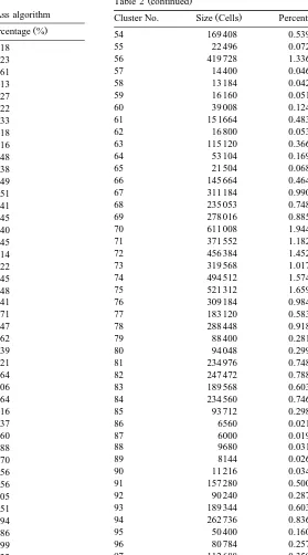
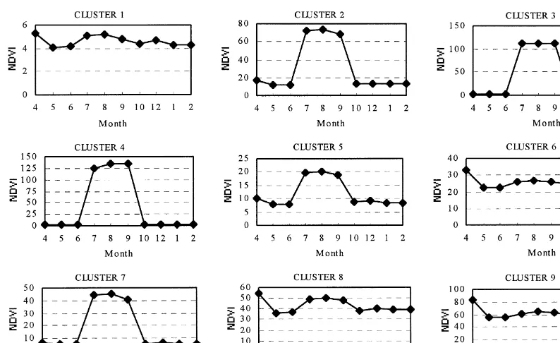
. standard deviation of the 10-month NDVI and graphics for each of the 100 clusters were calculated and visualised. As an example, Table 2 shows the size of each cluster and Fig. 3 shows the mean values of the 10-month NDVI for 9 of the 100 clusters.
Referring to these results, the statistic character-istics of monthly NDVI images, and the available
Ž
conventional data landuse map of China, resources and environment data of China, GTOPO30, ground
.
truth data, etc. , the clustering result was comprehen-sively analysed and the clusters with single land-cover classes were identified. For the clusters with mixed landcover classes and size more than 1.0% of the total pixels, unsupervised clustering was carried out again. The identified clusters with single land-cover were combined. The remaining clusters were combined into one mixed cluster.
Table 2
Size of each cluster calculated by theISOCLASSalgorithm
Ž . Ž .
Cluster No. Size Cells Percentage %
1 5520 0.018
27 289 280 0.921
28 1 025 648 3.264
29 1 415 840 4.506
30 1 120 032 3.564
31 539 312 1.716
32 1 205 680 3.837
33 1 087 120 3.460
34 310 448 0.988
35 619 152 1.970
36 363 104 1.156
37 771 680 2.456
38 692 768 2.205
39 298 752 0.951
40 720 720 2.294
41 246 960 0.786
42 596 688 1.899
43 635 216 2.022
44 602 960 1.919
45 488 768 1.555
46 550 928 1.753
47 474 592 1.510
48 701 104 2.231
49 570 352 1.815
50 674 976 2.148
51 438 000 1.394
52 321 456 1.023
53 137 680 0.438
Ž .
Table 2 continued
Ž . Ž .
Cluster No. Size Cells Percentage %
54 169 408 0.539
55 22 496 0.072
56 419 728 1.336
57 14 400 0.046
58 13 184 0.042
59 16 160 0.051
60 39 008 0.124
61 15 1664 0.483
62 16 800 0.053
63 115 120 0.366
64 53 104 0.169
65 21 504 0.068
66 145 664 0.464
67 311 184 0.990
68 235 053 0.748
69 278 016 0.885
70 611 008 1.944
71 371 552 1.182
72 456 384 1.452
73 319 568 1.017
74 494 512 1.574
75 521 312 1.659
76 309 184 0.984
77 183 120 0.583
78 288 448 0.918
79 88 400 0.281
80 94 048 0.299
81 234 976 0.748
82 247 472 0.788
83 189 568 0.603
84 234 560 0.746
85 93 712 0.298
91 157 280 0.500
92 90 240 0.287
93 189 344 0.603
94 262 736 0.836
95 50 400 0.160
96 80 784 0.257
97 112 688 0.359
98 204 864 0.652
99 116 176 0.370
100 187 312 0.596
Total 31 422 573 100
likeli-Fig. 3. Mean values of the 10-month NDVI of China for the first nine clusters.
hood algorithm was used to separate the mixed cluster.
4.3. LandcoÕer dataset and map
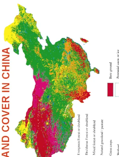
Finally, the landcover dataset of China was gener-ated with 11 classes that are described in Table 3. Fig. 4 shows a landcover map of China with legend.
4.4. Accuracy assessment
Vegetated surfaces change seasonally based on the composition of the vegetation present. Past inves-tigations have demonstrated that classes developed from multitemporal NDVI data represent characteris-tic patterns of seasonality and correspond to relative
Ž
patterns of productivity Loveland et al., 1991; Brown .
et al., 1993 . Thus, it is reasonable to use monthly NDVI data through the year to identify seasonal
Ž .
greenness Chen, 1998 . However, experience has shown that at least 60% of the seasonal greenness
Ž
classes represent multiple landcover types Brown et .
al., 1993; Running et al., 1995 . This is the result of
spectral similarities between some natural and agri-cultural landcover types. These problems can usually be solved by developing criteria based on the rela-tionship between the confused seasonal greenness classes and selected ancillary datasets.
To correctly perform classification accuracy as-sessment, it is necessary to compare two sources of
Ž .
information: 1 the remote-sensing-derived classifi-Ž .
cation map and 2 what we will call reference test
Table 3
Derived landcover dataset of China
Value Landcover class
0 Sea
14 Evergreen Forest or shrubland 70 Deciduous Forest or shrubland 120 Mixed forest or shrubland 132 Natural grasslandrpasture
140 Grass crops
170 Wetland
180 Little vegetation
191 Bare ground
200 Perennial snow or ice
Fig.
4.
Landcover
in
Ž . information which may in fact contain errors . The relationship between these two sets of information is commonly summarised in an error matrix.
Information in the error matrix may be evaluated
Ž . Ž .
using 1 simple descriptive statistics andror 2 discrete multivariate analytical statistical techniques. By using the simple descriptive statistics technique,
oÕerall accuracy is computed by dividing the total Ž
correctly classified pixels sum of the major diago-.
nal by the total number of pixels in the matrix.
KAPPA analysis is a discrete multivariate technique
Ž
of use in accuracy assessment Congalton and Mead, .
1983; Jensen, 1996 . KAPPA analysis yields a Khat
Ž .
statistic an estimate of KAPPA that is a measure of Ž
agreement or accuracy Rosenfield and Fitzpartrick-.
Lins, 1986; Congalton, 1991 . The Khat statistic is computed as the number of observations in row i and column i,
xiq and xqi are the marginal totals for row i and column i, respectively, and N is the total number of observations.
A training dataset produced by combining ground truth data and the data collected randomly from the landuse map of China and the resources and environ-ment data of China, was used to assess the accuracy of the landcover classification. The error matrix of the classification was analysed by using the training dataset. The calculated overall accuracy was 91.3%, while K was equal to 89.4%.
Based on the accuracy assessment, most land-cover classes were successfully classified. The classes with disparate seasonal greenness characteristics, like those with vegetation and without vegetation, are easily separated. However, the classes with similar seasonal greenness characteristics such as natural grasslandrpasture and gross crops, bare ground and perennial snow or ice, are difficult to separate. The accuracy limitation of this landcover classification has mainly resulted from the use of limited channels of satellite data, i.e., NDVI only, and ancillary data.
5. Conclusions
A landcover dataset for the whole of China is very useful for many applications, especially in global change research, land resources development and management, natural disaster monitoring and damage evaluation, and can support decision making for sustainable development. While the 1-km landcover dataset of China produced in this study is currently the best available, the accuracy of the dataset and the details of landcover classification were limited be-cause the classification was performed by using only NDVI and limited ancillary data.
To refine this product, it will be necessary to improve this derived landcover dataset by using more ancillary data, such as DTM, more ground truth data, field survey results, data derived from higher
resolu-Ž .
tion satellite data e.g., Landsat TM, SPOT, etc. , and other landcoverrlanduse maps. Also it would be better to attempt this procedure using all five chan-nels of AVHRR information as much as possible rather than only NDVI derived from channel 1 and channel 2. This will also make it be possible to produce a landcover dataset with landcover classes as many as those described in the LCWGrAARS Landcover Classification System. In addition, the authors suggest the development of an integrated database to assess the results and integrate the datasets in a GIS so that they can be conveniently used by various users.
Appendix A. The LCWGrrrrrAARS landcover clas-sification system
Value Landcover Class
10 Vegetation
12 Forest or shrubland
36 Needleleaf
60 Forest and shrubland 70 Deciduous
110 Forest and shrubland 120 Mixed forest or shrubland
130 Grassland
132 Natural grasslandrpasture 140 Grass crops
141 Paddy
142 Wheat
143 Sugarcane
144 Corn
146 Wheat and rice
157 Other
160 MixedÕegetation
170 Wetland
172 Mangrove
174 Swamp
180 LittleÕegetation
182 Tundra
184 Other
190 Non-vegetation
191 Bare ground
192 Rock
193 Stones or gravel
194 Sand
195 Clay
200 Perennial snow or ice
210 Built-up area
220 Water
222 Inland water
224 Water with seasonal change 226 Tidal flat
References
Blaisdell, E.A., 1993. Statistics in Practice. Harcourt Brace Jo-vanovich, New York.
Brown, J.F., Loveland, T.R., Merchant, J.W., Reed, B.C., Ohlen, D.O., 1993. Using multisource data in global land-cover char-acterization: concepts, requirements, and methods.
Photogram-Ž .
metric Engineering and Remote Sensing 59 7 , 977–987. Chen, X., 1997. Analysis on Land Cover Change and Its Impacts
on Sustainable Development based on Remote Sensing and GIS: A Case Study in Ansan, Korea. Technical Report, Sys-tems Engineering Research Institute, Korea Institute of Sci-ence and Technology, Taejon, Korea.
Chen, X., 1998. Developing Methodologies and Datasets of Multi-resolutionr-temporal LanduserCover Classification in China with Satellite Data and SIS: Potential and Programs. Technical Report, Center for Environmental Remote Sensing
ŽCEReS , Chiba University, Japan..
Chen, X., Hu, H., 1999. Evaluation on algorithms for land cover classification from landsat TM data in Ansan, Korea.
Asian-Ž .
Pacific Remote Sensing and GIS Journal 11 1 , 52–57. Congalton, R.G., 1991. A review of assessing the accuracy of
classifications of remotely sensed data. Remote Sensing of
Ž .
Environment 37 1 , 35–46.
Congalton, R.G., Mead, R.A., 1983. A quantitative method to test for consistency and correctness in photointerpretation.
Pho-Ž .
togrammetric Engineering and Remote Sensing 49 1 , 69–74.
Ž
Earth Resources Mapping, 1995. ER Mapper Reference Vers.
.
5.0 . Earth Resources Mapping Pty. Ltd., Perth, Australia. Foody, G.M., Campbell, N.A., Trood, N.M., Wood, T.F., 1992.
Derivation and applications of probabilistic measures of class membership from the maximum-likelihood classification.
Pho-Ž .
togrammetric Engineering and Remote Sensing 58 9 , 1335– 1341.
Haralick, R.M., Fu, K., 1983. Pattern recognition and
classifica-Ž .
tion. In: Colwell, R. Ed. , Manual of Remote Sensing. Ameri-can Society of Photogrammetry, Falls Church, VA, pp. 793– 805.
Jensen, J.R., 1996. Introductory Digital Image Processing — A Remote Sensing Perspective. 2nd edn., Prentice-Hall, Engle-wood Cliffs, NJ.
Loveland, T.R., Merchant, J.M., Ohlen, D.O., Brown, J.F., 1991. Development of a land-cover characteristics database for the conterminous US. Photogrammetric Engineering and Remote
Ž .
Sensing 57 10 , 1453–1463.
Moody, A., Strahler, A.H., 1994. Characteristics of composited AVHRR data and problems in their classification.
Interna-Ž .
tional Journal of Remote Sensing 15 17 , 3473–3491. Rosenfield, G.H., Fitzpartrick-Lins, K., 1986. A coefficient of
agreement as a measure of thematic classification accuracy.
Ž .
Running, S.W., Loveland, T.R., Pierce, L.L., Nemani, R.R., Hunt, E.R., 1995. A remote sensing based vegetation classification logic for global land cover analysis. Remote Sensing of
Envi-Ž .
ronment 51 1 , 39–48.
Schalkoff, R., 1992. Pattern Recognition: Statistical, Structural and Neural Approaches. Wiley, New York.
Swain, P.H., Davis, S.M., 1978. Remote Sensing: The Quantita-tive Approach. McGraw-Hill, New York.