Rapid Quantitative Imaging of High-Intensity Ultrasound Pressure Fields." Journal of the Acoustical Society of America. The lower figure on the right shows the position of the displacement maps shown on the left in the larger phantom, superimposed on a full-FOV axial image.
Motivation
However, MR thermometry has the disadvantages of resulting in tissue heating and unwanted bioeffects (Wang et al., 2014) when FUS is applied for its non-thermal applications in the brain. 3D MR-ARFI scans ( de Bever et al., 2016 ) are capable of encoding an entire brain volume in two dimensions, but result in long scan times due to increased phase encoding steps.
Dissertation Synopsis
Relatively long scan times of MR-ARFI methods maintain a low FUS duty cycle to encode a volumetric view that can cover the entire focus in transcranial FUS applications. The proposed 3D MR-ARFI technique with a reduced FOV shows a long tube that can cover the entire focal spot.
Ultrasound Basics
Ultrasound Propagation
Reflection and Transmission
The greater the difference in impedance at the boundary, the greater the reflection that will occur, the smaller the amount of energy that will be transferred. However, reflection can result from the interface between soft tissue and bone at the normal incidence of the wave and total reflection of the longitudinal wave at angles greater than 25◦.
Attenuation
In general, when the angle of incidence is not too large, the ultrasound beam suffers little from reflection due to the small difference in impedance values when it penetrates from one soft tissue to another. The average soft tissue absorption coefficient ranges from 3 to 5 m-1MHz-1, except for the tendon and testicles, which have absorption coefficients of 14 and 1.5 m-1MHz-1, respectively.
Effects of Ultrasound on Tissues
Thermal Effects
Nonthermal Effects
- Cavitation
- Acoustic radiation force
For example, the peak of the acoustic radiation field is located close to the focal point of the acoustic field (Palmeri and Nightingale, 2011). In highly damping materials, the acoustic radiation force is distributed more evenly, so the peak does not appear near the focal point.
Ultrasonic Field Measurement
Hydrophone
Unlike piezoelectric types, fiber optic hydrophones are based on the optical principles that the refractive index in a liquid is modulated by an ultrasonic field (Hocker, 1979; Phillips, 1980; Gopinath et al., 2007). Compared to piezoelectric types, fiber-optic hydrophones can withstand higher pressure levels, are easy to repair, and have long-term stability and flat and wide bandwidth (Parsons et al., 2006).
Radiation Force Balance Measurements
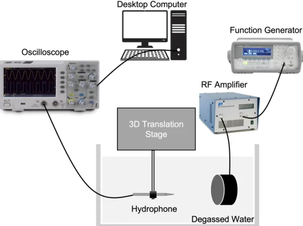
Ultrasonic field mapping is performed in a test tank and the hydrophone is connected to a 3D translation stage for mechanical scanning of the acoustic field, as Figure 2.2 illustrates. Here, M is the sensitivity of the hydrophone, the value of which is selected at the frequency of the ultrasound direction in the frequency response graph.
Schlieren Visualization
Cross-correlation of two background images with and without light diffraction could produce refractive index maps. BOS imaging has been used to qualitatively describe the acoustic field in 2D (Butterworth and Shaw, 2010) and 3D (Pulkkinen et al., 2017).
Applications of Therapeutic Focused Ultrasound
A Brief History
Finally, the inverse Radon transform and an approximate method were used to calculate the 3D pressure field (Pulkkinen et al., 2017). By 1992, MRI was first combined with FUS to guide and monitor tissue damage (Yang et al., 1992), which prompted the development of therapeutic use.
Applications
- Neuromodulation
- Blood-Brain Barrier Opening
After the procedure, BBB disruption is verified by MR contrast imaging (Kinoshita et al., 2006) with intravenous injection of gadolinium contrast. In addition, several clinical studies (Abrahao et al., 2019; Mainprize et al., 2019) further demonstrated the safety and efficacy of FUS to open the BBB in humans.
Magnetic Resonance Imaging (MRI)
MR Physics
- Magnetization, Precession and Relaxation
- Spatial Localization and K-Space
- Constrained MR Undersampled Reconstruction
- Structured Low-Rank Approaches for MR Reconstruction
The direction of the main field B0(z) is the longitudinal direction while the other two dimensions (xy) perpendicular to the z dimension are the transverse direction. The transverse component of the magnetization causes the flux in the receiver coil (mostly the same coil that generates the RF field) to change, and then the coil can detect the precursor magnetization as MR signals.
MRI for Guiding Focused Ultrasound
MR Thermometry
The nuclear standard can be minimized by calculating the abbreviated singular value decomposition (SVD) (Haldar, 2013; Shin et al., 2014). Moreover, an additional phase shift can be caused by intense gradient use (El-Sharkawy et al., 2006).
MR Acoustic Radiation Force Imaging
Some tricks, such as using unbalanced gradients (de Bever et al., 2016) and internal volume imaging (Schneider et al., 2013) can reduce 3D scan times and image the FUS beam with contiguous slices. Furthermore, MR-ARFI sequences can be modified to allow simultaneous measurement of temperature-induced PRF shift and ultrasound-induced displacement, which has been reported in (Auboiroux et al., 2012; Viallon et al., 2010; Qiao et al., 2020). Apart from FUS localization, MR-ARFI can assess tissue stiffness for ablative applications (Vappou et al., 2018; Hertzberg et al., 2014).
Abstract
Introduction
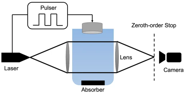
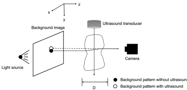
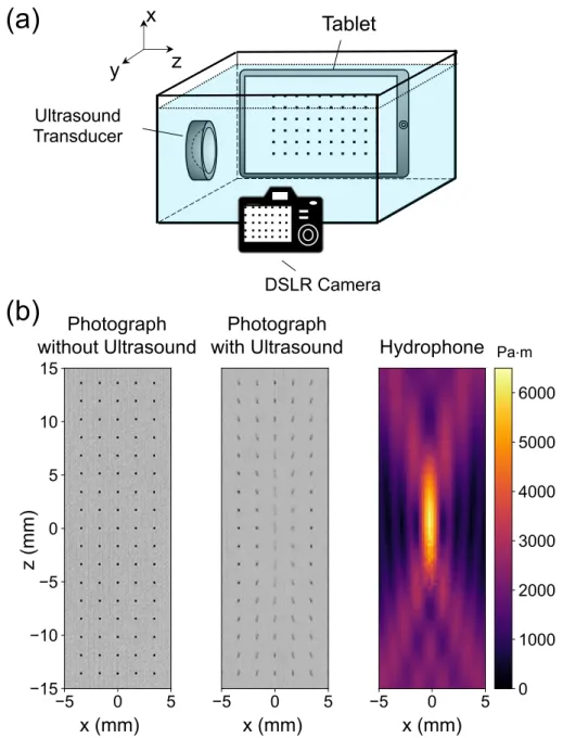
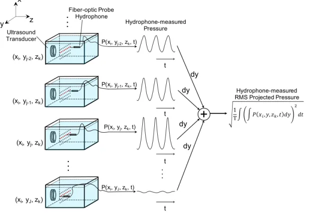
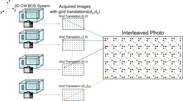
To obtain the same maps with a hydrophone, 3D hydrophone measurements along the line-of-sight dimension are integrated to obtain projected pressure waveforms, and then the RMS amplitude of the projected waveform is calculated, as illustrated on the right. When FUS is turned on, the nails fade in a characteristic pattern related to the projected pressure at each spatial location in the photograph. a) A 2D CW-BOS system consists of a glass tank filled with water acoustically coupled to the transducer, a tablet displaying a background pattern, and a camera to photograph the blurred pattern. The method was implemented and compared with fiber optic hydrophone RMS projected pressure measurements, to evaluate its feasibility, accuracy and robustness.
Methods
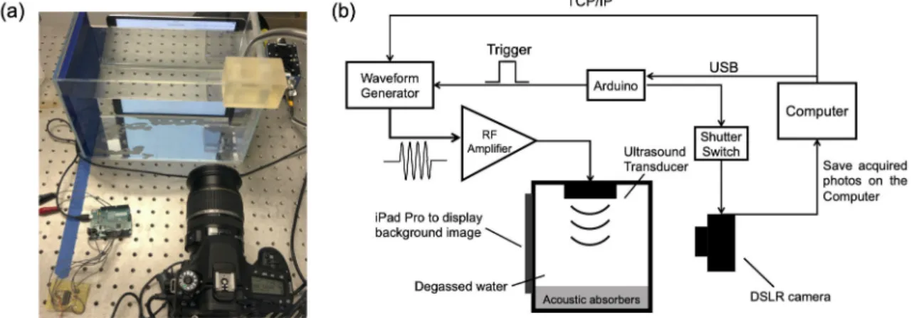
- Optical and FUS Hardware Setup
- CW-BOS Acquisition Details
- Optical Hydrophone Measurements
- Mathematical Model for CW-BOS Imaging of FUS Pressure Fields
- Numerical FUS Beam Simulations and Training Data Generation
- Neural Network Architecture and Training
A single high-resolution RMS projected pressure map (0.425 x 0.425 mm2) was calculated from the 16 photos as described below. The training data for the reconstructor included simulated CW-BOS histograms paired with their RMS-predicted pressure amplitudes. The ccc coefficient vector was the input to the neural network which derived the projected RMS pressure value corresponding to that histogram, as illustrated in Figure 3.6 and described further below.
Results
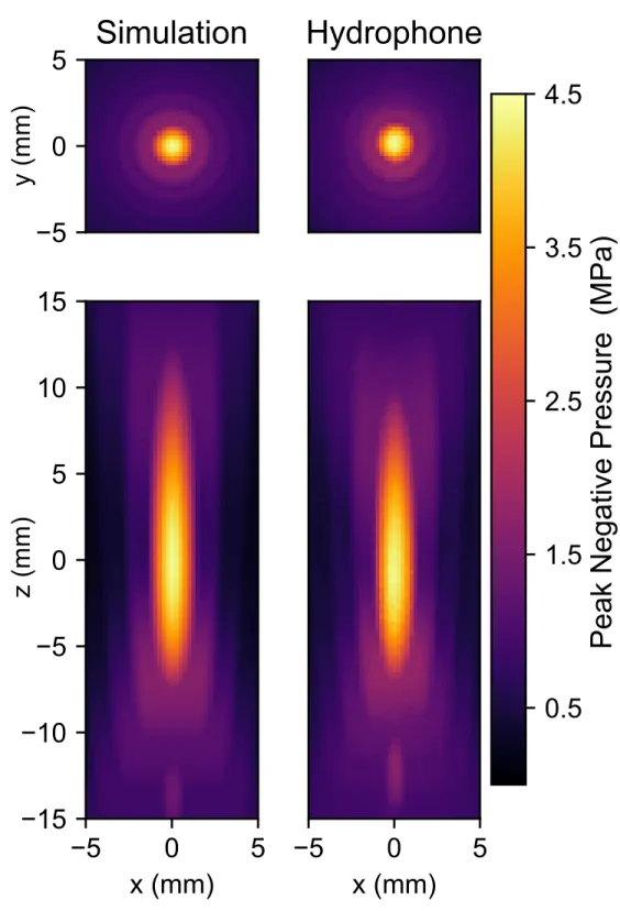
- Comparison of FUS Beam Simulations and Hydrophone Measurements
- Two FUS Frequencies
- Pressure Amplitude
- Signal-to-Noise Ratio and Number of Averages
- Rotation and Translation
- Aberrations
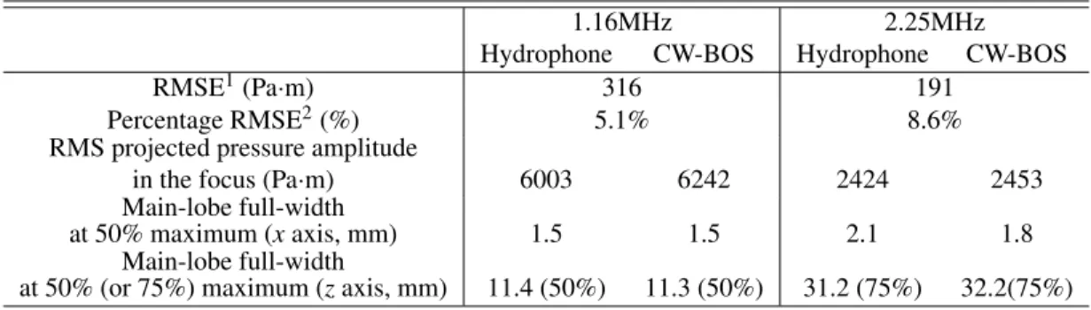
The map resulting from eight averages is the maximum shown in Figure 3.10a, which was indistinguishable from the map resulting from the maximum ten averages (not shown). The CW-BOS RMS projected beammap, hydrophone beammap measured with this aberrator configuration and their difference are shown in Figure 3.12b. The difference in the maximum RMS projected pressure is 236 Pa·m (11.7% of the hydrophone measured peak amplitude).
Conclusions
To make it portable, the tank can be sealed, the tablet and camera can be rigidly attached to it, and the FUS can be attached to it via a mylar membrane. This is a parameter that can be optimized: Moving the beam closer to the background pattern would magnify the blur patterns by a factor<1, which would allow for a larger field of view at the cost of reduced sensitivity. At the same time, the storage space required for each network was small (<1 MB), so many networks could be trained and stored, and the most suitable one could be selected for each map.
Acknowledgments
Although the proposed CW-BOS hardware is not currently compatible with very large aperture transcranial FUS transducers whose focus does not extend beyond their shell, it is possible to map these systems by projecting background patterns onto the transducer surface. The beam propagation direction is from bottom to top. a) Measured maps and their difference for the 1.16 MHz converter. An aberrator made of silicon was placed in front of the lower half of the 1.16 MHz transducer.
Abstract
Introduction
Thus, the FUS-duty cycle of the MR-ARFI should be kept as low as possible. Existing MR-ARFI sequences are either 2D, 2D reduced-FOV, or 3D, where 3D methods ( de Bever et al., 2016 ) encode an entire brain volume in two dimensions. The phantom and in vivo brain results show that the proposed MR-ARFI scan recovered the FUS focus with high reliability compared to full sampling.
Methods
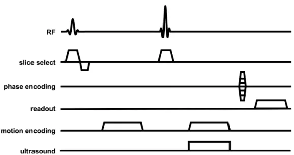
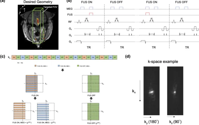
Pulse Sequence
To reduce scan time, scanning used a small EPI factor with uniform subsampling in the phase-coded EPI dimension and PF sampling in the other phase-coded dimension. The acquired k-space data of the xON+ and xON- images were uniformly subsampled in the ky direction with an acceleration factor (R) of 2 with complementary sampling patterns. Fractional Fourier (PF) encoding was used in the kz-direction to further reduce the scan time by a factor of 0.67.
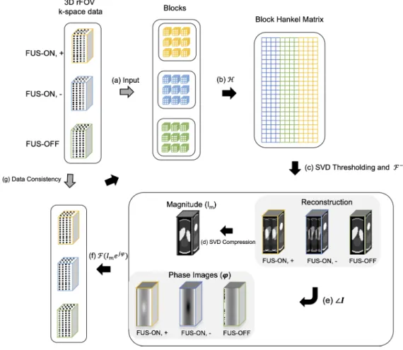
Image Reconstruction
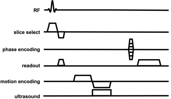
The FUS emission was synchronized with the first MEG (odd kylins) or second MEG (even kylins) ( Mougenot et al., 2015 ). The timing of ultrasound emission was alternated between odd and even kylines to obtain complementary k-space data between the two FUS-ON images. In addition, the FUS-ON and FUS-OFF k-space data sets were acquired with opposite PF directions to obtain complementary k-space data (FUS-ON: 'left half', FUS-OFF: 'right half' in Figure 4.1 c).
Experiments
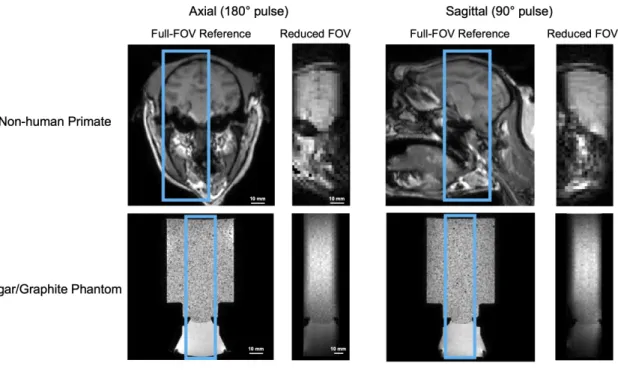
A pair of 2-channel phased-array coils (Flex-L; Philips Healthcare) was placed on either side of the phantom. A pair of dual-channel phased-array coils (Flex-S; Philips Healthcare) was placed on either side of the macaque's head. Mean (±standard deviation) displacements at peak displacement, maximum displacement, and full width at half maximum (FWHM) of the displacement profiles along the US-x/y/z direction were calculated.
Results
The reconstruction algorithm failed in this case due to the lack of the FUS-OFF image's k-space data in the joint reconstruction. The axial slice shown on the right illustrates the location of the focus and sub-images on a full-FOV reference image. The second row shows a reconstruction from retrospective undersampling of the fully sampled data set and the third row shows a reconstruction from a prospective undersampled scan.
Discussion
We found that too large a PF factor can lead to blurring of focus in the z-dimension; at the same time, using an opposite PF sampling pattern in the FUS-OFF acquisition mitigated this blurring. However, significant “dead time” remained in the scan (specifically, nearly 450 ms of each 500 ms TR) that could be used for additional data acquisition at the expense of reduced signal due to reduced longitudinal relaxation between excitations. Shorter FUS pulses would also enable a shorter TE in the sequence, which would further increase the SNR.
Conclusion
If off-resonance was not a concern, the EPI factor could be increased and the scan time would be shortened in proportion to that increase. 8 ms MEGs and FUS pulses with a 0.85% duty cycle were used in this work, yielding peak displacement phase shifts of approximately 0.20 radians in the phantom scans and 0.18 to 0.24 radians in the macaque scans. For example, if the duty cycle can be increased or if the pulses can be driven with higher power and shortened, additional FUS-ON measurements can be made in the same scan time which can allow reduction in the PF factor or the undersampling (R ) factor, without compromising the displacement phase shift.
Acknowledgements
The axial plane was selected with a 180◦RF pulse and the sagittal plane with a 90◦RF pulse. The right image shows the position of the magnified displacement maps on the left in the axial plane (US x-y) of the whole brain. The right image shows the position of the magnified displacement maps on the left in the axial plane (US x-y) of the whole brain.
Summary and Contributions
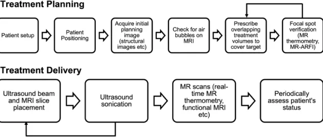
Considering the effects of distorted or shifted waves, we need to image a view that can cover the entire focus for the success of treatment with MRI. The 'dead' time in the long TRs was used for the alternative acquisition of FUS-ON and FUS-OFF data, with a complementary k-space sampling pattern. This will improve the efficiency of targeting the FUS focus for finding, redirecting and phase correction of the focus.
Future Work
CW-BOS System for Rapid FUS Beam Mapping
The partial Fourier sampling and uniform subsampling were performed in two phase-encoding dimensions, which minimized the FUS duty cycle and further reduced scan times. It will optimize the routine to calibrate the ultrasound transducer, detect the aberrated ultrasound beams and check the agreement between different experiments. For example, ultrasound beam maps with and without skull aberration in ex vivo can be obtained with the established system, and the relationship between two maps can be studied for acoustic properties of the skull.
Reduced-FOV 3D MR-ARFI
Histological safety of transcranial focused ultrasound neuromodulation and magnetic resonance acoustic radiation force imaging in rhesus macaques and sheep. Adaptation of MRI acoustic radiation force imaging for in vivo human brain focused ultrasound applications. Magnetic resonance in medicine. MRI detection of the thermal effects of focused ultrasound on the brain. Ultrasound in medicine and biology.