We conclude this study by the spontaneous formation of transverse waves along the wave front of. The remaining data are taken in the shock-normal direction and are evenly spaced along the blast front.
Detonation wave structure
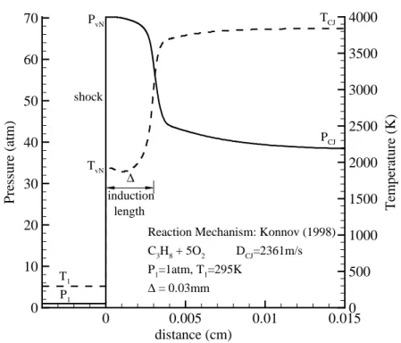
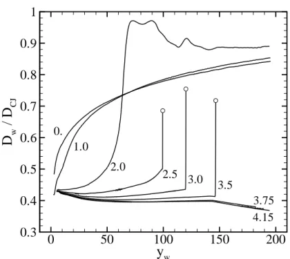
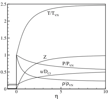
The induction length ∆ depends on the post-shock conditions and the details of the chemical kinetics. Overdriven detonations (D > DCJ) are also possible when the particle velocity u > uCJ at the end of the reaction zone.
Detonation diffraction
Experimental observations
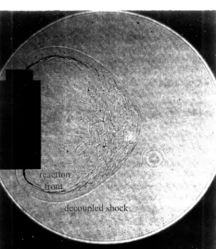
Whether a diffractive burst will propagate successfully (supercritical diffraction, Fig. 1.6) or not (subcritical burst, Fig. 1.7) is the result of several factors, namely, the composition of the reactive, thermodynamic mixture. the condition of the undisturbed reactants, the degree of detonation overload, and the geometrical setup of the experiment. Two distinct modes of restart have been identified by Murray and Lee (1983): "spontaneous" in the bulk of the reactive mixture; and "with reflection", on the boundary walls.
Direct numerical simulations
These cells weakened as soon as they propagated into the lower layer, while new transverse waves spontaneously formed along the shock front, moved toward the dilution region, and ignited the unburned shocked reactants. Vorticity appears to provide a strong coupling mechanism between the two orthogonal modes and is probably the triggering mechanism for the production of new transverse waves.
Thesis outline
We investigate the mechanism of spontaneous generation of transverse waves due to reflection of the unstable rarefaction front. The sum of the thermality coefficients σK in equation (2.4) expresses the total pressure change as a result of chemical reaction at constant volume.

Reactive Euler equations in intrinsic coordinates
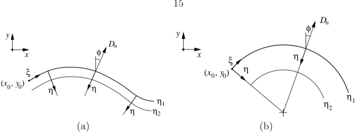
B expresses the rate of change of arc length with respect to a fixed reference axis as measured by an observer always moving in the normal direction of impact. can be expressed as a function of curvature and normal impact velocity, B = . 2.12). The expression B0(t) represents the final angle between the impact normal and the reference axis.
The Lagrangian derivative of temperature
In equation (2.18), κs(t) andDs(t) are the precurvature and shock velocity evaluated on the axis of symmetry. Such regions are the channel symmetry axis and the corner wall, i.e. the two boundary regions of a diffracting wave front.
Quasi-steady, quasi-one-dimensional reaction zone
The relationship between Dn and κ can be found by solving a two-point boundary value problem with a regularity condition at the sonic point (Klein et al. 1995). Downstream of the sonic point, the solution can be supersonic or subsonic, and the flow is similar to expanding or compressing isentropic flow in a divergent nozzle.

The reaction mechanism
The chapter closes with the description of the initial and boundary conditions of the problem. The variables are not dimensionalized taking as reference the uniform conditions upstream of the shock (subscript 0).
Numerical integration
Parallel implementation
Boundary conditions are implemented on the sides of the patch by priming a boundary layer of guard cells with the appropriate values. These functions hide the inner workings of the concurrent implementation to the rest of the application.
Shock and flow gradient tracking
The algorithm begins by locating the peak density along the symmetry axis of the channel. Once this position is identified, the first grid point on the left (in the reaction zone) is taken as the starting point for a downward search of the computational grid. At each grid point of the scan sequence, the y-gradient of density is evaluated by a standard centered difference formula and compared to a threshold value.
Lagrangian particles
Lagrangian particles integration
Particle trajectory integration is performed by the Predictor-Corrector method in the form of an Adams-Bashforth (P) predictor followed by an Adams-Moulton (C) corrector. The general scheme is of the PECE type, where step E shows the updating of the derivative part from the last calculated value (in Numerical Recipes 1992, pp. 747–751). This information is sent to all other processors (slaves) at the beginning of an integration step and collected by the master at the end of the integration.
Computational setup
- Boundary conditions
- Initial conditions
- Low activation energy
- High activation energy
- Intermediate activation energy
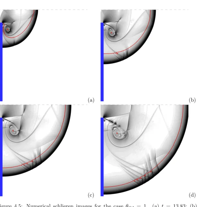
Changing θCJ changes the rate of energy release in the ZND profile and the sensitivity of the reaction rate to variations in the thermodynamic state. Large values of the activation energy result in a chemical reaction rate that is very sensitive to changes in the thermodynamic state. The very low pressures in the region of the corner cause the shock to initially propagate at much lower speeds along the wall than along the axis.
High-resolution studies
- Particle analysis
As the vortex rotates clockwise, it wraps around it a contact discontinuity (CD1) produced by the acceleration of the flow at the corner. To the left of the RS, the transmitted shock (TS) is curved due to expansion outside the channel. This separation can be compared to the reference length 10 ∆1/2, in the lower corner of the plot.
- Particle analysis
This structure is shown in figure 4.16, where the flow field behind the contact discontinuity CD2 is very similar to the flow shown in fig. The position of the leading shock, Z = 0.05 and Z = 0.95 reaction loci, and the sonic line at the channel axis are plotted in Fig. We now discuss the results obtained for a selection of particles injected along the channel axis (Fig. 4.18).
- Particle analysis
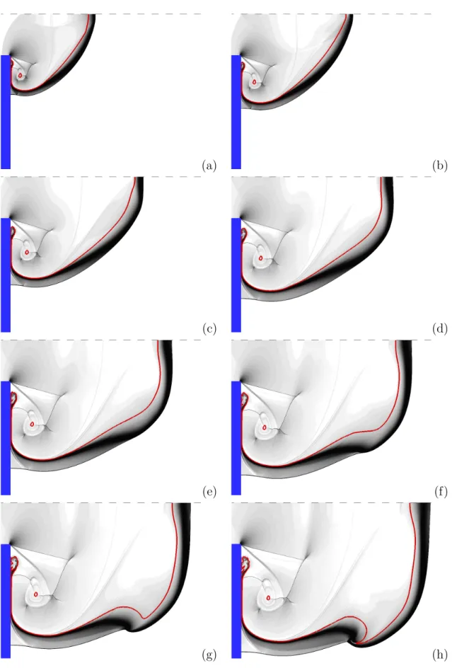
Each frame is a close-up of the computational domain, near the leading shock, at the symmetry axis of the channel. However, no acceleration of the front can be observed at the axis of symmetry in fig. Along the axis of symmetry (Fig. 4.27), at the arrival of the expansion, the shock velocity decreases and a small delay is formed between the shock and the 0.05 locus.
Conclusions: a failure model for diffraction
Another variation in DT /Dt is linked to the arrival of the transverse wave att ~= 43. These facts suggest that a vanishing Lagrangian derivative of temperature at post-shock conditions is the criterion for the local decoupling of the shock front from the reaction zone ,. In Section 5.1 we use Skews's construction for a diffraction-free non-reactive shock and compare his calculation of the perturbation angle with the value estimated from the present simulations.
Detonation asymptotics
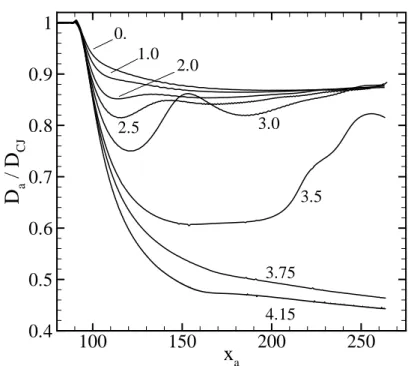
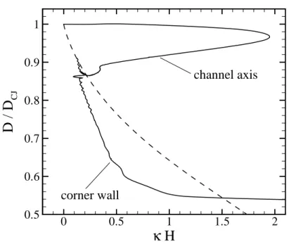
Due to the overlapping system of transverse waves at the end of the simulation, the main reaction region along the symmetry axis cannot be reduced to a quasi-one-dimensional, quasi-stationary solution. Interestingly, at a distance of about 6H, the calculated Dn–κ curve approaches the lower end of the quasi-stationary curve shown in the figure. Because of the progressive separation of the shock from the reaction zone, this problem is closer to explosion breakdown than detonation.
Reduction to blast equation
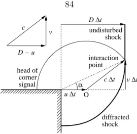
No part of the curve from the simulation can be approximated by a straight line passing through the origin. If we estimate that the initial explosion radius is the x-distance from the vertex to the arrival point of the angular signal, then. However, the above derivation ignores the reactivity of the current, so that it is independent of the reaction mechanism.
Whitham shock dynamics
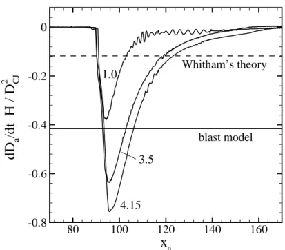
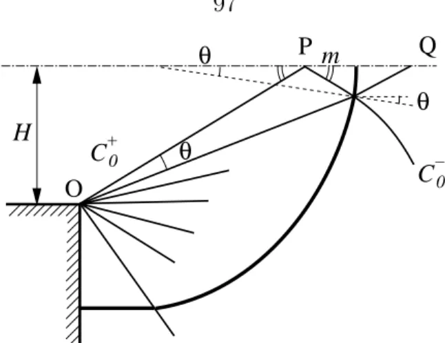
4.3, where subcritical explosions exhibit a wall impact velocity of about 40% of the initial value of CJ. The deceleration of the axial stroke, after reflecting the first characteristic, is found in the limit of δθ → 0 by comparing the decrease in speed from M0 to Ma with the time to travel the distance P Q,. Since κd is exactly twice the curvature in the axis at the moment preceding the reflection of the first characteristic, we see that in fact a second discontinuity in the curve propagates along C0−.
Closure of the failure model
Since Q ∼ DCJ2, equation (5.40) is also a comparison of the chemical time scale of the order of magnitude 1/k with the gas dynamic time scale of the order Da/D˙a. We state that if equation (5.40) is verified downstream of this point, the shock–reaction decoupling will continue until the reaction is stopped. The trigger for the formation of these waves is shock reflection in the early stages of detonation cornering, as explained in Section 4.2.1: the foot of the shock lags behind the undisturbed detonation front and is reflected from the wall at an angle.
Computational setting
The concept of an acoustic channel for disturbances traveling in the transverse direction of the main shock is also introduced. We find that waves are amplified in the reaction zone depending on the reaction order and activation energy, and that the amplification takes place preferentially along contact discontinuities where the sonic parameter reaches a local maximum. In Section 6.5, the amplitude of a transverse wave is tracked in time and its exponential growth is related to the gain coefficient found in Section 6.3.
Non-reactive reference case
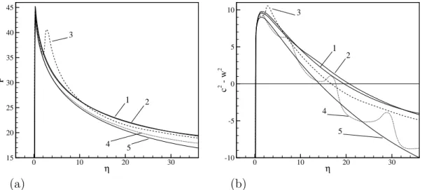
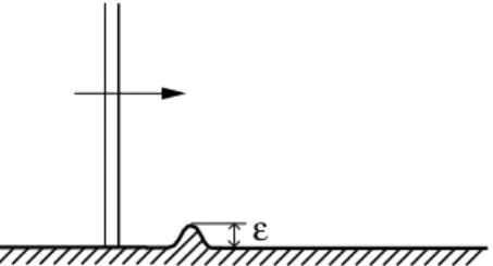
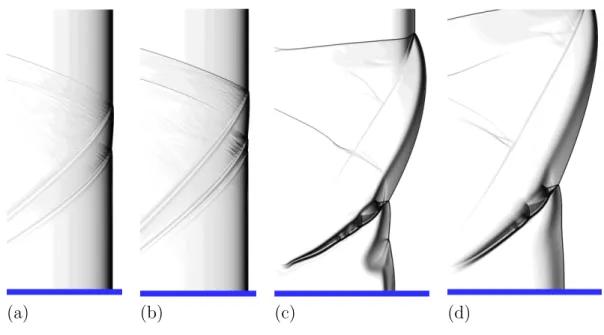
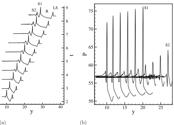
Because Schlieren imaging amplifies every ripple in a numerical simulation, we take four horizontal slices of the computational domain at the locations indicated in frame (a) and show quantitative profiles in frame (b). On the scale of the graph, the pressure oscillations are very small and their wavelength is about ², the only length scale in this non-reactive problem. The results obtained by Strehlow and Fernandes (1965) and Barthel and Strehlow (1966) for infinitesimal, high-frequency, transverse perturbations in a planar ZND detonation are presented in the next section.
Linear acoustic theory
The coefficient l and m= (1−l2)1/2 are the cosines of direction with respect to the axis η, in the direction of detonation propagation, and ξ, in the transverse direction. Since Zk is found by solving equation (6.4), the above result does not depend on the specific energy release function DZ/Dt, and is also valid when the detonation is overdriven. The last term in square brackets of equation (6.9) represents the negative contribution due to wave spreading, i.e. the separation of acoustic beams infinitely close to the beam.

Comparison of different reaction models
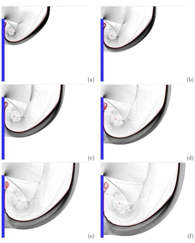
The changes in flow caused by the obstacle are much smaller in the non-activation energy calculations, Fig. 6.6 (a) and (b). The only immediately obvious difference between the two calculations is that the third contact discontinuity appears only in the simulation of the second-order reaction. The dashed lines corresponding to the 50% reaction completion locus provide a visual indication of the actual extent of the reaction zone in the Schlieren images.
Growth of transverse waves
The inner box is a close-up of the plot showing the fluctuations in the detonation velocity at the wall. We perform a convergence study of the structure of the triple point observed in the case θCJ = 3.5 (Fig. 4.25). The number of cells in the reference half-reaction zone (the segment shown at the lower left of the pressure plot) is 22.5.
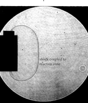
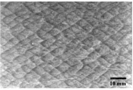
Sooted aluminum sheet. From Kaneshige (1999)
Temperature and pressure profile for a ZND wave as a function of the
Mole fraction profile for a ZND wave
Sonic parameter for a ZND wave
Schematic of a diffracting shock (Skews’ construction)
Intrinsic coordinates ξ and η for an arbitrary front, (a), and specialized
Comparison of unsteady term evaluations. Solid line: Equation (2.19)