Many load balancing schemes rely on the availability of global knowledge about the load distribution in a system. Furthermore, the degradation of the load balancing process provides control over the degree to which this locality is maintained. Many methods require all the computers involved to go through the load balancing phase simultaneously.
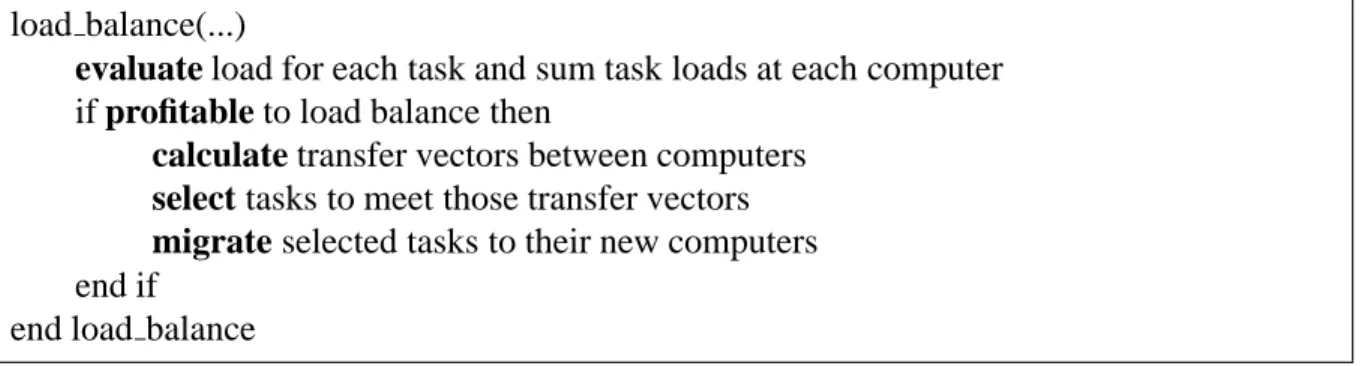
Once the loads of the computers are measured, the presence of a load imbalance can be detected. If the cost of the imbalance exceeds the cost of load balancing, load balancing must be initiated. Indeed, many of the current load balancing algorithms fail to fully address several of the above concerns.
Methodology
- Load Evaluation
- Analytic Load Evaluation
- Empirical Load Evaluation
- Hybrid Load Evaluation
- Load Balance Initiation
- Load Imbalance Detection
- Profitability Determination
- Work Transfer Vector Calculation
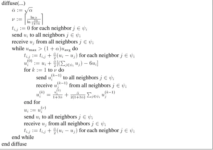
- Heat Diffusion
- Gradient Methods
- Hierarchical Methods
- Domain-Specific Methods
- Task Selection
- Task Transfer Options
- Task Selection Algorithms
- Other Constraints
- Task Migration
- Summary
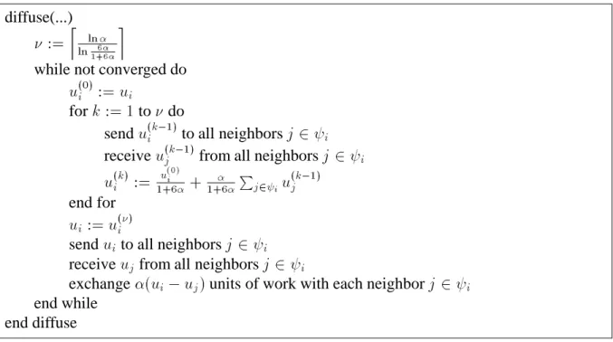
To adapt the routines for torus-free meshes, simply replace the load on the computer at the mesh boundary with the loads of its non-existing neighbors. Unfortunately, the time discretization error in (2.3) is O() (i.e., the scheme is first-order time-accurate). As shown in equation (2.6), the Crank-Nicholson scheme is equivalent to repeated multiplication of the original vector u(0) by the matrix A;1B.
This has the advantage of eliminating much of the cost of transferring the load through intermediate computers. However, if the average workload of the task is high relative to the size of the transfer vectors, it can be very difficult to achieve a good load balance. Basically what the algorithm does is create a list of possible candidates for it. optimal subset, removing those subsets whose sums are "close" to those of other subsets.
Note that if E(R(C)) < E(C), the current configuration always changes. Importantly, it is possible to change the configuration with higher power consumption.) If the current configuration does not change for some time, T is updated via S. In such circumstances, only a subset of the tasks on the computers in question may need to be considered.
Implementation
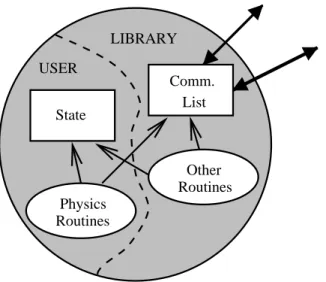
The Concurrent Graph Library
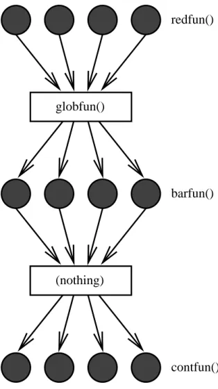
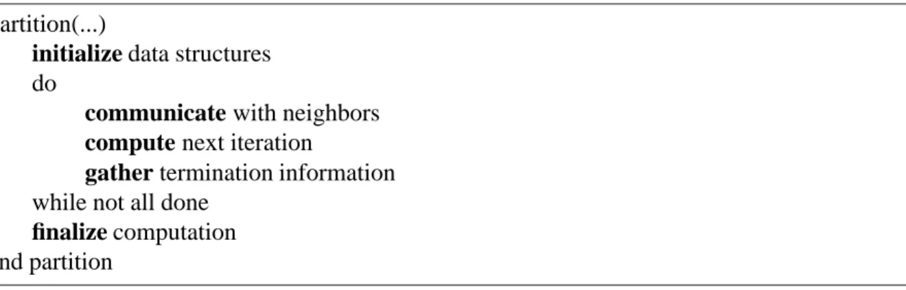
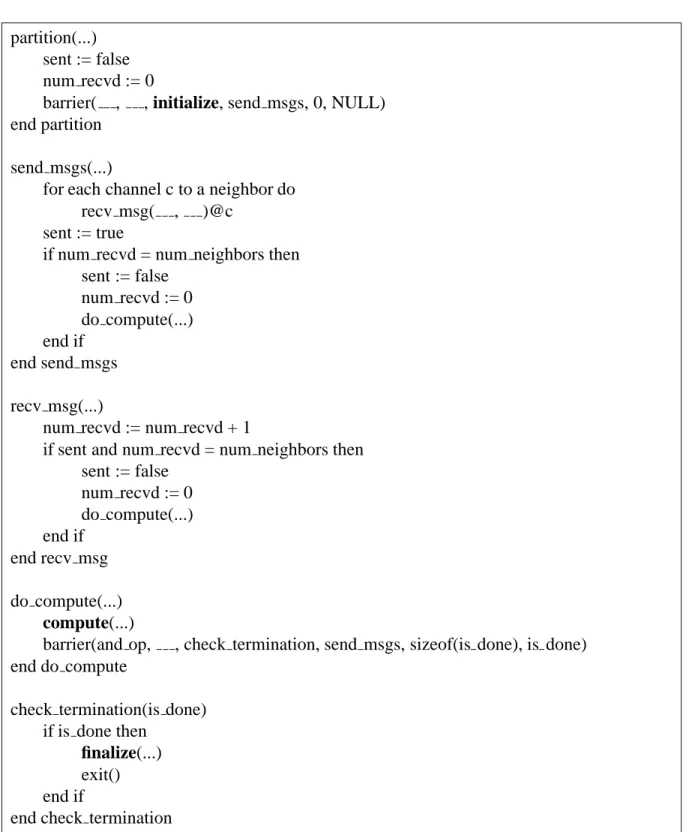
The user part consists of the state of the node and the routines that operate on it. The library part consists of a communication list and helper routines such as load balancing and visualization functions. The global function globfun is called on the null computer with the result of the reduction (this provides an easy way to output a break condition or a "begin time step" message, for example).
When this function completes, the barrier function barfun (if any) is called on each node with the result of the reduction operation. A function executed using node-to-node RPC executes to completion without blocking or interrupting. The special form of the barrier() function is due to its typical use in scientific applications.
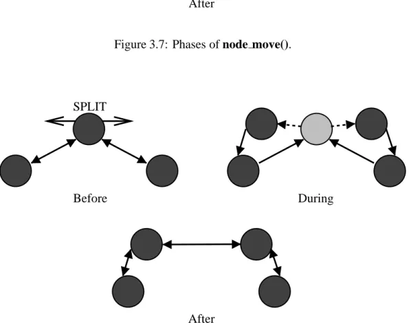
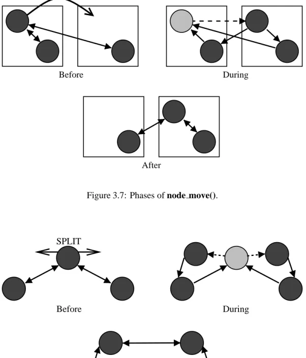
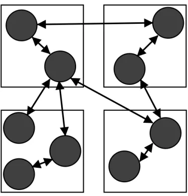
That is, moving a node from one computer to another affects only those two computers, plus any computers that contain nodes that communicate with the node that was moved. Similarly, the node dividing and combining routines affect only the computer on which the node(s) reside, plus the computers that contain adjacent nodes in the graph. The node move() function moves the given node from the current computer to the specified computer, as shown schematically in Figure 3-7.
The node split() function splits a given node into two nodes—a process illustrated in Figure 3.8. Upon splitting, the original node becomes a ghost node that forwards every RPC that arrives to the appropriate child node. The other node remains as it is and incorporates the other node's state information into its own.
When a procedure call arrives at the old, now ghost node, it forwards the message to the new, now combined node, then tells the message sender to change its communication channels appropriately.
Implementation Specifics
- Low-Latency RPC Mechanism
- Load Evaluation
- Load Balance Initiation
- Work Transfer Vector Calculation
- Node Selection
- Node Migration
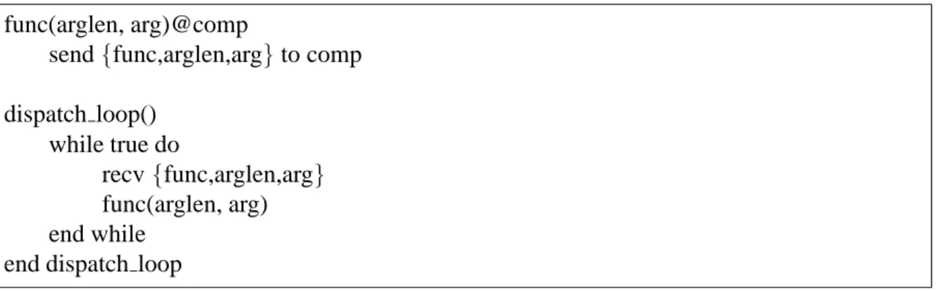
You can access information about the computer's load using the load balancing routines to determine when and how to balance the load. A diagram of an instrumented RPC dispatch routine between computers is given in Figure 3.11. Depending on whether the used hash table is unique for a specific node or is global for all nodes in the computer, functions (or their classes) can be timed for each node separately or for all nodes within the computer or
The Graph Library also provides a basic set of node load functions that can be provided to the load balancing routine. The above load measurement techniques are only a good basis for load balancing decisions if past load is a good predictor of future load (that is, the load on nodes and the computers on which they are assigned is not drastically changes with respect to the frequency of division of labor). After globfun() completes, the barfun() barrier function is called on each node with the result of the reduce operation.
The initial value ofui is the computer's load, calculated in the previous step, and the value ofis1;mine. Nodes are selected to satisfy a transfer vector using a combination of the methods in Chapter 2. The node selection process is repeated using these markers to satisfy the portion of the transfer vectors that have not yet been satisfied from previous selection steps.
When all transfer vectors are less than this minimum possible difference, no more node markers will be moved and the algorithm will terminate. This is, of course, a very weak bound on the time for completion - in practice, this stage requires a number of exchanges roughly proportional to the severity of the imbalance and the diameter of the mesh.). Note that it is possible for a marker to move an arbitrary distance from its original PC (ie, the movement is completely unbounded).
If a node does not move for this reason, it is marked as "still" and the load balancing process restarts from the initial load balancing phase.
Final Algorithm
Experiments
- Direct Simulation Monte Carlo Application
- Description
- Results
- Particle-in-Cell Application
- Description
- Results
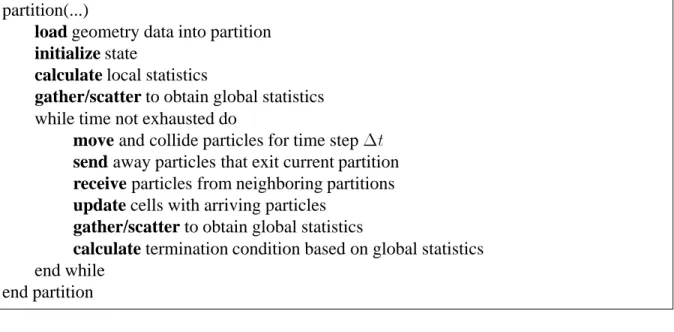
The DSMC algorithm implemented on each partition of the problem is given in Figure 4.1. As stated in the description of the DSMC technique, collisions within each partition (and the grid cells within it) are calculated independently. As described in the description of the GEC grid above, just over 50 percent of the grid cells actually contain particles.
Consequently, one would expect that a standard spatial decomposition and mapping of the grid would result in a very inefficient computation. The electromagnetic effect of each particle relative to the vertices of the lattice cell containing the particle is calculated. Once the field solver has converged, the effects of the new field are propagated back to the particles by adjusting their trajectories accordingly.
The state associated with a node consists of a portion of the grid and the particles in the corresponding portion of physical space. This boundary condition represents the fact that communication must be used to resolve an area of the field or transport particles. The physics routines used in Figure 4.6 describe the dynamics of particle motion and the solution of the field.
As a result, slow ions are pushed out of the beam and move back towards the spacecraft. Closer examination reveals that this deficiency is due to the two-phase nature of the PIC code. As a result, the total load of these two phases on a given computer does not balance the individual phases of the computation.
The above examples suggest that what one needs is a load balancing strategy that balances each phase of the computation collectively. Note that the characteristics of the PIC code also imply that one must generally allocate multiple partitions to each computer. A cut-off in the middle will balance the total load, but none of the component phases will be balanced.
Alternative Methodologies
Conclusion
This thesis demonstrates that a practical, comprehensive approach to load balancing is possible and effective, but it also shows that considerable work remains to be done. In particular, while a simple scalar approach to load balancing is useful for applications involving a single phase of computation, the method does not achieve high efficiency for computations consisting of multiple phases, each with different load distribution characteristics. Dynamic granularity control via task customization and improved software interfaces would reduce the burden on the application developer.
The PIC code experiments in Chapter 4 clearly demonstrate the limitations of the scalar view of loading. Although the load balancing algorithm apparently achieved a good balance of the total load of each computer, it failed to balance the components of the load. Thus, single-block approaches (which include most techniques in the literature) are doomed to failure. 2) Use load balancing to encourage task/node scaling.
Task-based load balancing strategies fail when the load of a single task exceeds the average load across all computers. Both the first- and second-order accurate schemes converge slowly as a function of the size of the mesh network. 47 . gence becomes particularly slow as high-frequency components of the load distribution are damped, exposing low-frequency components.
Introducing asynchrony into the load balancing process would allow its cost to overlap with idle time on underloaded computers and would not break applications that do not have algorithmic synchronization points. While the load balancing software interface is quite simple—the user only needs to provide routines to pack and unpack a task's state—further improvements could be made. In addition, the data structure libraries should be modified to support automatic unpacking and packaging of hte structures into them, better supporting checkpointing, load balancing, and routine message passing.
Consequently, a multi-component vector will undoubtedly be required to adequately characterize the load.
Bibliography
Runtime and language support for compiling adaptive irregular issues on machines with distributed memory.” Software: Practice. Numerical simulation of ion beam plume backflow for spacecraft contamination assessment. PhD Dissertation, MIT Aeronautics and Astronautics Department, 1995. Three-dimensional plasma particle-in-cell calculations of ion thruster backflow contamination.” Submitted to the Journal of Computational Physics, 1995.