eAppendix to “Effect Decomposition in the Presence of Treatment-induced Confounding: A
Regression-with-Residuals Approach”
Geoffrey T. Wodtke
*University of Chicago
Xiang Zhou Harvard University
*Direct all correspondence to Geoffrey T. Wodtke, Department of Sociology, University of Chicago, 1126 E. 59th Street, Chicago, IL 60637; email: [email protected].
1 Derivation of Parametric Expressions for the rNDE and rNIE under Linear Models for M and Y
Under assumptions (i) to (iii) and the assumption that equations
E(M|C,A) = θ0+θ1TC⊥+θ2A (1) E(L|C,A) = τ0+τ1TC⊥+τ2A (2) E(Y|C,A,L,M) = β0+βT1C⊥+β2A+βT3L⊥+β4M+β5AM (3)
from the main text are all correctly specified, the rNDE is equal to rNDE=
∑
c
∑
m
∑
l
[E(Y|c,a∗,l,m)P(l|c,a∗)−E(Y|c,a,l,m)P(l|c,a)]P(m|c,a)P(c)
=
∑
c
∑
m
∑
l
[(β0+βT1c⊥+β2a∗+βT3l⊥+β4m+β5a∗m)P(l|c,a∗)−
(β0+βT1c⊥+β2a+βT3l⊥+β4m+β5am)P(l|c,a)]P(m|c,a)P(c)
=
∑
c
∑
m
[(β0+βT1c⊥+β2a∗+βT3E(L−E(L|c,a∗)|c,a∗) +β4m+β5a∗m)−
(β0+βT1c⊥+β2a+βT3E(L−E(L|c,a)|c,a) +β4m+β5am)]P(m|c,a)P(c)
=
∑
c
∑
m
[(β0+βT1c⊥+β2a∗+β4m+β5a∗m)−
(β0+βT1c⊥+β2a+β4m+β5am)]P(m|c,a)P(c)
=
∑
c
∑
m
[(β2a∗+β5a∗m)−(β2a+β5am)]P(m|c,a)P(c)
=
∑
c
[(β2a∗+β5a∗E(M|c,a))−(β2a+β5aE(M|c,a))]P(c)
=
∑
c [(β2a∗+β5a∗(θ0+θ1Tc⊥+θ2a))−(β2a+β5a(θ0+θ1Tc⊥+θ2a))]P(c)= (β2a∗+β5a∗(θ0+θ1TE(C−E(C)) +θ2a))−(β2a+β5a(θ0+θ1TE(C−E(C)) +θ2a))
= (β2a∗+β5a∗(θ0+θ2a))−(β2a+β5a(θ0+θ2a))
= [β2+β5(θ0+θ2a)](a∗−a),
2
and the rNIE is equal to rNIE=
∑
c
∑
m
∑
l
[P(m|c,a∗)−P(m|c,a)]E(Y|c,a∗,l,m)P(l|c,a∗)P(c)
=
∑
c
∑
m
∑
l
[P(m|c,a∗)−P(m|c,a)](β0+βT1c⊥+β2a∗+βT3l⊥+β4m+β5am)×
P(l|c,a∗)P(c)
=
∑
c
∑
m
[P(m|c,a∗)−P(m|c,a)](β0+βT1c⊥+β2a∗+βT3E(L−E(L|c,a∗)|c,a∗)+
β4m+β5a∗m)P(c)
=
∑
c
∑
m
[P(m|c,a∗)−P(m|c,a)](β0+βT1c⊥+β2a∗+β4m+β5a∗m)P(c)
=
∑
c
∑
m
[(β0+βT1c⊥+β2a∗+β4m+β5a∗m)P(m|c,a∗)−
(β0+βT1c⊥+β2a∗+β4m+β5a∗m)P(m|c,a)]P(c)
=
∑
c
[(β0+βT1c⊥+β2a∗+E(M|c,a∗)(β4+β5a∗))−
(β0+βT1c⊥+β2a∗+E(M|c,a)(β4+β5a∗))]P(c)
=
∑
c
[(E(M|c,a∗)−E(M|c,a)](β4+β5a∗)P(c)
=
∑
c
[(θ0+θ1Tc⊥+θ2a∗)−(θ0+θ1Tc⊥+θ2a)](β4+β5a∗)P(c)
=
∑
c
(θ2a∗−θ2a)(β4+β5a∗)P(c)
=θ2(β4+β5a∗)(a∗−a).
2 Analytic Standard Errors for Regression-with-residuals
In this appendix, we outline an approach to obtaining analytic standard errors for regression- with-residuals estimates of the rNDE and rNIE. With this approach, we assume that the variables{C,A,L,M,Y} satisfy the Causal Markov assumption, that is, we assume that they are represented by a recursive system of equations with independent errors.1 Let X denote a p×1 vector of ones, the treatment A, baseline confounders centered at their sample means ˆC⊥ , and any interactions between A and ˆC⊥; let L denote aq×1 vector of post-treatment confounders; and finally, letZdenote ar×1 vector containing the me- diator M and any of its interactions with X. A “naive” least squares regression of the outcomeYon{X,L,Z}can be expressed as follows:
Y=αˆTX+ηˆTL+γˆTZ+Yˆ⊥
=αˆTX+
∑
j
ηˆjLj+γˆTZ+Yˆ⊥, (4)
where Lj is the jth element of L and ˆY⊥ denotes the residual. Similarly, a least squares regression of eachLjonXcan be expressed as follows
Lj =λˆTj X+Lˆ⊥j , (5) where ˆL⊥j denotes the residual.
Substituting (5) into (4) yields the following expression for the outcome:
Y= (αˆT+
∑
j
ˆ
ηjλˆTj)X+
∑
j
ˆ
ηjLˆ⊥j +γˆTZ+Yˆ⊥. (6)
Since ˆY⊥ is the least squares residual for regression (4), it is orthogonal to the span of {X,L,Z}. Because each ˆL⊥j is a linear combination ofX and Lj, {X, ˆL⊥,Z} and{X,L,Z} span the same space. Thus, equation (6) represents the least squares fit ofYon{X, ˆL⊥,Z}, meaning that ˆαTRWR = (αˆT+∑
j
ˆ
ηjλˆTj )are the regression-with-residuals estimates of the co- efficients on treatment, the baseline confounders, and any interactions between them, ˆη
4
are the regression-with-residuals estimates of the coefficients on the post-treatment con- founders, and ˆγ are the regression-with-residuals estimates of the coefficients on the mediator and any of its interactions with treatment and/or the baseline confounders.
Therefore, the asymptotic variance-covariance matrix for the regression-with-residuals estimates(η, ˆˆ γ) can be obtained directly via conventional methods after fitting the naive regression (4).
The asymptotic variance-covariance matrix for ˆαRWR can be obtained with the delta method. Given the assumption thatYand Lhave mutually independent errors, each ˆλjis independent of ˆαand ˆη. The variance-covariance matrix for ˆαRWR can then be estimated as
Vˆ(αˆRWR) =Vˆ(αˆ) +Covd(α, ˆˆ η)ΛˆT+ΛˆVˆ(ηˆ)ΛˆT+
∑
j,k
ηˆjηˆkCovd(λˆj, ˆλk), (7) where ˆΛ= [λˆ1, ˆλ2, ..., ˆλq]is ap×qmatrix of estimated coefficients from model (5),V(·)is the variance-covariance matrix of a random vector, and Cov(·,·)is the covariance matrix between two random vectors. In equation (7), the first three terms can be obtained directly from the naive regression (4), and the covariance matrix between ˆλjand ˆλkin the last term can be estimated as
Covd(λˆj, ˆλk) = (lˆ⊥j )Tlˆ⊥k
n−p (XTX)−1, (8) wherenis the sample size, and ˆl⊥j and ˆl⊥k aren×1 vectors of the residualized confounders Lˆ⊥j and ˆL⊥k . Similarly, the covariance matrix between ˆαRWRand ˆγcan be estimated as
Covd(αˆRWR, ˆγ) =Covd(α, ˆˆ γ) +ΛˆCovd(η, ˆˆ γ). (9) Now consider the plug-in estimators of the rNDE and rNIE. Without loss of gener- ality, assume that a∗−a = 1. Given that the error terms for equations (1) and (3) are independent, asymptotic variances forrNDE and\ rNIE can be estimated using the delta[
method2:
Vˆ[rNDE\] =Vˆ(βˆ2) + (θˆ0+θˆ2a)2Vˆ(βˆ5) +βˆ25Vˆ(θˆ0+θˆ2a) + (θˆ0+θˆ2a)Covd(βˆ2, ˆβ5) (10) Vˆ[rNIE[] = (βˆ4+βˆ5a∗)2Vˆ(θˆ2) +θˆ22Vˆ(βˆ4+βˆ5a∗). (11)
In these equations, the terms involving ˆθ0 and ˆθ2 can be estimated by applying equa- tions (7-9) to the regression-with-residuals model (1) from the main text, and the terms involving ˆβ2, ˆβ4, and ˆβ5can be estimated by applying equations (7-9) to the regression- with-residuals model (3) from the main text.
6
3 Derivation of Parametric Expressions for the rNDE and rNIE under a Nonlinear Model for M
When the mediator is binary or counts, a generalized linear model may be preferred for estimatingE[M|A,C]. Under assumptions (i) to (iii) and the assumption that both this mediator model and the outcome model (3) from the main text are correctly specified, then the rNDE conditional onC=cis equal to
rNDE(c) =
∑
m
∑
l
[E(Y|c,a∗,l,m)P(l|c,a∗)−E(Y|c,a,l,m)P(l|c,a)]P(m|c,a)
=
∑
m
∑
l
[(β0+βT1c⊥+β2a∗+βT3l⊥+β4m+β5a∗m)P(l|c,a∗)−
(β0+βT1c⊥+β2a+βT3l⊥+β4m+β5am)P(l|c,a)]P(m|c,a)
=
∑
m
[(β0+βT1c⊥+β2a∗+βT3E(L−E(L|c,a∗)|c,a∗) +β4m+β5a∗m)−
(β0+βT1c⊥+β2a+βT3E(L−E(L|c,a)|c,a) +β4m+β5am)]P(m|c,a)
=
∑
m
[(β2a∗+β5a∗m)−(β2a+β5am)]P(m|c,a)
= [(β2a∗+β5a∗E(M|c,a))−(β2a+β5aE(M|c,a))]
= [β2+β5E(M|c,a)](a∗−a)
and the rNIE conditional onC=cis equal to rNIE(c) =
∑
m
∑
l
[P(m|c,a∗)−P(m|c,a)]E(Y|c,a∗,l,m)P(l|c,a∗)
=
∑
m
∑
l
[P(m|c,a∗)−P(m|c,a)](β0+βT1c⊥+β2a∗+βT3l⊥+β4m+β5am)P(l|c,a∗)
=
∑
m
[P(m|c,a∗)−P(m|c,a)](β0+βT1c⊥+β2a∗+βT3E(L−E(L|c,a∗)|c,a∗)+
β4m+β5a∗m)
=
∑
m
[P(m|c,a∗)−P(m|c,a)](β0+βT1c⊥+β2a∗+β4m+β5a∗m)
=
∑
m
[(β0+βT1c⊥+β2a∗+β4m+β5a∗m)P(m|c,a∗)−
(β0+βT1c⊥+β2a∗+β4m+β5a∗m)P(m|c,a)]
= [(β0+βT1c⊥+β2a∗+E(M|c,a∗)(β4+β5a∗))−
(β0+βT1c⊥+β2a∗+E(M|c,a)(β4+β5a∗))]
= (β4+β5a∗)[E(M|c,a∗)−E(M|c,a)].
8
4 Empirical Illustration with a Binary Outcome
In this section, we present a parallel analysis of the NLSY79 in which the outcome,Y, is coded as a binary variable for illustrative purposes. Specifically,Y is coded 1 if a respon- dent scored in the top quintile of the CES-D distribution, indicating he or she is among the most depressed 20% of the population, and 0 otherwise. All other variables are de- fined as in Section 4 from the main text. We use the following models for the mediator and outcome:
E(M|C,A) = θ0+θ1TC⊥+θ2A+θ3C⊥A (12) E(Y|C,A,L,M) = β0+βT1C⊥+β2A+βT3L⊥+β4M+β5AM+β6C⊥A, (13)
where E(Y|C,A,L,M) = P(Y = 1|C,A,L,M) and thus our model for the outcome is a linear probability model. To estimate the rNDE and rNIE, we first compute residuals for each of the baseline confounders C and post-treatment confounders L, which involves centering the elements of Caround their sample means and centering the elements of L around their estimated conditional means given the past. Specifically, we estimate condi- tional means for each post-treatment confounder from a linear regression that includesC, A, and all two-way interactions between them. We then compute least squares estimates of equations (12) and (13), and finally, we use their coefficients to construct regression- with-residuals estimates of the rNDE, rNIE, and rATE.
Consistent with our analysis of continuous scores from the CES-D, results based on the binary measure described previously also suggest that completing a post-secondary education has a sizable overall effect on the risk of depression. Specifically, completing college is estimated to lower the risk of depression by 7.7 percentage points (95% CI:
[-0.129,-0.021]). The rNDE is estimated to be -0.058 (95% CI: [-0.105, -0.003]), which sug- gests that attending college would still reduce the risk of depression by 5.8 percentage points even after an intervention to fix the income distribution to that observed when nobody receives a post-secondary education. The rNIE is estimated to be -0.020 (95% CI:
[-0.042,-0.003]. This suggests that, if everyone already attended college, the risk of depres-
sion would be further reduced by only about 2 percentage points after an intervention to shift the income distribution to that observed when everyone attends college from that observed when nobody attends. Estimates of the rNDE and rNIE provide some mini- mal evidence of mediation, although they are fairly imprecise, as indicated by their wide confidence intervals.
These results are based on a linear probability model for the outcome. As with any model, researchers should consider the possibility of bias due to misspecification and take steps to avoid it (e.g., by using regression diagnostics, interaction terms, model selection techniques, and subject matter knowledge). With a linear model for a strictly bounded outcome, researchers should take additional precautions to ensure that it is a reasonable approximation for the true conditional expectation function and does not suffer from se- vere misspecification. For example, with a linear probability model, researchers should confirm that it does not yield many nonsensical predictions well outside the logical[0, 1] range.
10
5 Simulation Study of Bias due to Model Misspecification
Even when assumptions (i) to (iii) are satisfied, regression-with-residuals may still yield biased estimates if models for the outcome, mediator, and/or treatment-induced con- founders are incorrectly specified. In this section, we use a series of simulation experi- ments to investigate the sensitivity of regression-with-residuals to several types of model misspecification, including incorrectly modeled effect modification and non-linearity.
Specifically, we simulate n = 500 observations and estimate the rNDE and rNIE of a binary treatment A on a continuous outcome Y via a continuous mediator M in the presence of a baseline confounderC, a treatment-induced confounder L, and an “unob- served” variable U that affects both L and Y but not A or M. In each simulation, we generate these variables as follows: U ∼ N(µU = 0,σU = 1); C ∼ N(µC = 0,σC = 1); A|C ∼ Bernoulli(πA|C = Φ(−0.3+0.5C)); L|U,C,A ∼ N(µL|U,C,A = 0.5U+C(0.5− ηC) +A(0.5+αC),σL|U,C,A =1); M|C,A,L∼ N(µM|C,A,L =C(0.5−ηC) +A(0.5+αC) + 0.5(L−µL|C,A),σL|U,C,A = 1); and Y|U,C,A,L,M ∼ N(µY|U,C,A,L,M = 0.5U+C(0.5− ηC) +A(0.5+αC) + (L−µL|C,A)(0.5+λC) +M(1+γC−0.2A),σY|U,C,A,L,M=1). Here, Φis the standard normal cumulative distribution function;α is a parameter that controls the degree to whichCmodifies the effects ofAonL, M, andY;γis a parameter that con- trols the degree to whichCmodifies the effect ofMonY;λis a parameter that controls the degree to whichCmodifies the effect of LonY; and finally,ηis a parameter that controls whether the effects ofConL, M, andYare linear versus parabolic. In all simulations, the rNDE and rNIE are identified, and their true values are 0.5 and 0.4, respectively.
With these data, we implement regression-with-residuals exactly as outlined in Sec- tion 3.1. That is, in all simulations, we implement regression-with-residuals by fitting a model forLthat is linear and additive inAandC, a model forMthat is linear and additive inAandC, and a model forYthat is linear and additive inCand Lbut multiplicative in Aand M. These modeling constraints are satisfied in some simulations but not in others, as we vary the values of{α,γ,λ,η}to introduce different types of effect modification and non-linearity. We then evaluate the performance of regression-with-residuals in terms of its absolute bias, the magnitude of its absolute bias relative to the true effect of inter-
est, its root mean squared error (RMSE), and the magnitude of its RMSE relative to the RMSE of the regression-with-residuals estimator with correctly specified models, which are computed from 10,000 simulated datasets in each experiment.a
Table 1 presents results from a set of simulation experiments that evaluate the per- formance of regression-with-residuals when its models for L, M, and Y are incorrectly specified because the effects of treatment on these variables are constrained to be invari- ant when in fact they differ across levels ofC. The effects of Aon L, M, andYare made to differ across Cby varying the value of α from 0.0 to 0.5 while setting all other tuning parameters equal to zero. Whenα = 0.0, the effects of treatment are invariant, and there is no model misspecification. Whenα =0.5, by contrast, the unit-specific effects of treat- ment have a standard deviation as large as their mean, and models that constrain these effects to be invariant are badly misspecified. Results show that regression-with-residuals is biased for the rNDE and rNIE when its models for L, M, andY incorrectly constrain the effects of Ato be invariant inC, as expected. The magnitude of bias, however, is not especially large in this particular scenario.
Table 2 presents results from a second set of simulation experiments that evaluate the performance of regression-with-residuals when its model for Y is incorrectly specified because the effects of the mediator on the outcome are constrained to be invariant when in fact they differs across levels ofC. The effect of M onY is made to differ acrossC by varying the value of γfrom 0.0 to 0.5 while setting all other tuning parameters equal to zero. When γ = 0.0, the effect of the mediator is invariant, and there is no model mis- specification. Whenγ =0.5, the unit-specific effects of the mediator vary considerably in C, and thus an outcome model that constrains these effects to be invariant is badly mis- specified. Consistent with findings from Table 1, the results in Table 2 also demonstrate that regression-with-residuals is biased when its outcome model is misspecified, in this case because it incorrectly constrains the effects ofMonYto be invariant acrossC.
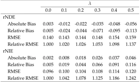
Table 3 presents results from a third set of simulation experiments that evaluate the performance of regression-with-residuals when its model for Y is incorrectly specified because the effects ofLonYare constrained to be invariant when in fact they differ across
aThe relative bias is computed as the ratio of the absolute bias to the true effect of interest.
12
Table 1: Misspecification bias in regression-with-residuals due to incorrectly modeled A→Y, A→ M, and A →Leffect modification byC
α
0.0 0.1 0.2 0.3 0.4 0.5
rNDE
Absolute Bias 0.003 0.009 0.020 0.026 0.034 0.046 Relative Bias 0.005 0.019 0.041 0.052 0.069 0.091 RMSE 0.140 0.142 0.142 0.143 0.144 0.148 Relative RMSE 1.000 1.016 1.012 1.018 1.029 1.053 rNIE
Absolute Bias 0.002 0.014 0.032 0.049 0.067 0.086 Relative Bias 0.005 0.035 0.079 0.121 0.167 0.216 RMSE 0.096 0.099 0.104 0.112 0.123 0.135 Relative RMSE 1.000 1.033 1.084 1.164 1.273 1.403
Note: Results are based on 10,000 simulations. Across all simulations,γ =0, λ =0, and η =0.
levels ofC. The effects ofLonYare made to differ acrossCby varying the value ofλfrom 0.0, in which case there is no effect modification, to 0.5, in which case the unit-specific effects of L have a standard deviation as large as their mean. As before, the remaining tuning parameters are all set to zero. Consistent with the results discussed previously, this set of simulations shows that regression-with-residuals is also biased when its outcome model incorrectly constrains the effects of L onY to be invariant across C, although the magnitude of this bias is fairly small across all scenarios.
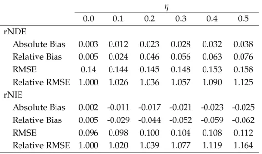
Finally, Table 4 presents results from a fourth set of simulation experiments that eval- uate the performance of regression-with-residuals when its models for L, M, andY are incorrectly specified because the effects ofC on these variables are assumed to be linear when in fact they are parabolic. The effects of C on L, M, andY are made to be nonlin- ear by varying the value of η from 0.0 to 0.5 while setting all other tuning parameters to zero. As η increases from zero, the effects of C become increasingly nonlinear, and the results in Table 4 show that regression-with-residuals becomes increasingly biased, as expected. Nevertheless, the bias due to non-linearity in these simulations is generally small. For reference, we also computed a set of naive regression estimates that do not
Table 2: Misspecification bias in regression-with-residuals due to incorrectly modeled M→Yeffect modification byC
γ
0.0 0.1 0.2 0.3 0.4 0.5
rNDE
Absolute Bias 0.003 -0.025 -0.048 -0.075 -0.099 -0.123 Relative Bias 0.005 -0.050 -0.096 -0.150 -0.198 -0.245
RMSE 0.140 0.143 0.148 0.161 0.176 0.195
Relative RMSE 1.000 1.024 1.060 1.150 1.259 1.390 rNIE
Absolute Bias 0.002 0.028 0.059 0.088 0.118 0.149 Relative Bias 0.005 0.070 0.147 0.221 0.296 0.373
RMSE 0.096 0.108 0.126 0.149 0.174 0.201
Relative RMSE 1.000 1.126 1.312 1.544 1.810 2.092
Note: Results are based on 10,000 simulations. Across all simulations,α =0, λ =0, and η =0.
Table 3: Misspecification bias in regression-with-residuals due to incorrectly modeled L→Yeffect modification byC
λ
0.0 0.1 0.2 0.3 0.4 0.5
rNDE
Absolute Bias 0.003 -0.012 -0.022 -0.035 -0.048 -0.056 Relative Bias 0.005 -0.024 -0.044 -0.071 -0.095 -0.113
RMSE 0.140 0.143 0.144 0.148 0.154 0.159
Relative RMSE 1.000 1.020 1.026 1.053 1.098 1.137 rNIE
Absolute Bias 0.002 0.008 0.018 0.026 0.037 0.046 Relative Bias 0.005 0.019 0.044 0.066 0.091 0.116
RMSE 0.096 0.100 0.104 0.108 0.114 0.120
Relative RMSE 1.000 1.042 1.078 1.125 1.186 1.242
Note: Results are based on 10,000 simulations. Across all simulations,α = 0, γ =0, and η =0.
14
Table 4: Misspecification bias in regression-with-residuals due to incorrectly modeled non-linearity in theC →Y,C → M, andC →Leffects
η
0.0 0.1 0.2 0.3 0.4 0.5
rNDE
Absolute Bias 0.003 0.012 0.023 0.028 0.032 0.038 Relative Bias 0.005 0.024 0.046 0.056 0.063 0.076
RMSE 0.14 0.144 0.145 0.148 0.153 0.158
Relative RMSE 1.000 1.026 1.036 1.057 1.090 1.125 rNIE
Absolute Bias 0.002 -0.011 -0.017 -0.021 -0.023 -0.025 Relative Bias 0.005 -0.029 -0.044 -0.052 -0.059 -0.062
RMSE 0.096 0.098 0.100 0.104 0.108 0.112
Relative RMSE 1.000 1.020 1.039 1.077 1.119 1.164
Note: Results are based on 10,000 simulations. Across all simulations,α = 0, γ =0, and λ =0.
adjust for the treatment-induced confounder L but that are otherwise based on correct models forE(M|C,A)andE(Y|C,A,M). These estimates suffer from bias due to uncon- trolled mediator-outcome confounding by Lbut not from bias due to effect modification or nonlinearity that has been incorrectly modeled, as above. Results from this ancillary analysis indicate that naive regression estimates understate the true rNDE by -0.165, or 32.9 percent, and that they overstate the true rNIE by 0.169, or 42.3 percent. Thus, in the simulations considered here where the magnitude of confounding is fairly large, bias arising from incorrect model specification is generally less severe than bias arising from uncontrolled mediator-outcome confounding.
6 Sensitivity Analysis for Unobserved Confounding
Assumptions (i) to (iii) require that there must not be any unobserved confounding of the treatment-outcome, treatment-mediator, or mediator-outcome relationships. The first two of these assumptions are similar to the conventional “exogeneity of treatment” as- sumption required in observational studies, where it is justified by adjusting for a suffi- cient set of baseline confounders, or in experimental studies, where it is met by design via random assignment. The third assumption, however, may fail to hold even in ran- domized experiments, and if unobserved confounding exists for the mediator-outcome relationship, regression-with-residuals estimates of the rNDE and rNIE will be biased. In this section, we outline a parametric approach to sensitivity analysis that permits an as- sessment of whether regression-with-residuals estimates are robust to violations of these three assumptions.
Consider the following set of linear structural equations characterizing the true causal relationships betweenA, M, andY:
A =γ0+γ1TC⊥+eA, (14)
M =θ0+θ1TC⊥+θ2A+eM, (15) Y =β0+βT1C⊥+β2A+βT3L⊥+β4M+β5AM+eY. (16) The assumptions of no unobserved confounding imply that the error terms (eA,eM,eY) are pairwise independent.
When the mediator-outcome relationship is confounded by unobserved factors (but not the treatment-outcome or treatment-mediator relationships),eMandeYare correlated.
A linear projection ofeY oneMcan be expressed as
eY =φMYeM+ψMY. (17)
Under the assumption thatE[ψMY|C,A,L,M] = 0, substituting (17) into (16) and taking
16
the conditional expectation ofYyields
E[Y|C,A,L,M] = (β0−φMYθ0) + (β1−φMYθ1)TC⊥+ (β2−φMYθ2)A+βT3L⊥+
(β4+φMY)M+β5AM. (18)
Thus, in this case, regression-with-residuals estimates of (β0,β1,β2,β4) suffer from an asymptotic bias ofφMY(−θ0,−θ1,−θ2, 1). Accordingly, the bias terms for the regression- with-residuals estimators of the rNDE and rNIE can be expressed as
Bias[rNDE] =−φMYθ2(a∗−a) (19) Bias[rNIE] =φMYθ2(a∗−a). (20) The biases for the rNDE and rNIE are equal in magnitude but opposite in direction. This implies that the overall effect, defined as the sum of the rNDE and rNIE, is not affected by unobserved mediator-outcome confounding, as expected. These expressions also imply that the rNIE, and thus the mediating role of M, will be overstated if φMY and θ2 are in the same direction and understated if they are in the opposite direction.
In practice, neither the sign nor the magnitude ofφMYis known. Moreover,φMYis not on an interpretable scale. To circumvent this problem,φMY can be re-expressed in terms of the correlation betweeneYandeMas follows:
φMY = sd(ψMY) sd(eM)
ρMY
q
1−ρ2MY
, (21)
whereρMY =Corr[eY,eM]. Substituting (21) into (19) yields
Bias[rNDE] =−θ2·sd(ψMY) sd(eM)
ρMY
q
1−ρ2MY
(a∗−a). (22) The bias for the rNIE can be expressed analogously. Under the assumptions of no unob- served treatment-mediator or treatment-outcome confounding,θ2, sd(eM), and sd(ψMY) can be consistently estimated from the mediator and outcome regressions described in
the main text. Thus, we can evaluate the bias terms as functions of ρMY and construct a range of bias-adjusted regression-with-residuals estimates for the rNDE and rNIE across different values ofρMY. In addition, we can identify the value ofρMYthat would suffice to reduce the estimated rNDE or rNIE to zero, or alternatively, the value that would suffice to render the estimated rNDE or rNIE statistically insignificant.
Next, consider the case where the treatment-outcome relationship is confounded by unobserved factors (but not the treatment-mediator or mediator-outcome relationships).
In this case,eAandeYare correlated, and a linear projection ofeY oneAcan be expressed as
eY =φAYeA+ψAY. (23)
Under the assumption thatE[ψAY|C,A,L,M] = 0, substituting (23) into (16) and taking the conditional expectation ofYyields
E[Y|C,A,L,M] = (β0−φAYγ0) + (β1−φAYγ1)TC⊥+ (β2+φAY)A+βT3L⊥+ β4M+β5AM.
Thus, in this case, regression-with-residuals estimates of(β0,β1,β2)suffer from an asymp- totic bias ofφAY(−γ0,−γ1, 1). Accordingly, the bias for the regression-with-residuals es- timator of the rNDE can be expressed as
Bias[rNDE] =φAY(a∗−a),
and because the treatment-mediator and mediator-outcome relationships are unconfounded, the regression-with-residuals estimator of the rNIE is asymptotically unbiased. As before, the bias for the rNDE can also be expressed as a function ofρAY =Corr(eA,eY):
Bias[rNDE] = sd(ψAY) sd(eA)
ρAY
q
1−ρ2AY
(a∗−a).
Finally, consider the case where the treatment-mediator relationship is confounded by unobserved factors (but not the treatment-outcome or mediator-outcome relationships).
18
In this case,eAandeMare correlated, and a linear projection ofeMoneAcan be expressed as
eM =φAMeA+ψAM. (24)
Under the assumption thatE[ψAM|C,A] = 0, substituting (24) into (15) and taking the conditional expectation ofMyields
E[M|C,A] = (θ0−φAMγ0) + (θ1−φAMγ1)TC⊥+ (θ2+φAM)A
In this case, regression-with-residuals estimates of (θ0,θ1,θ2) suffer from an asymptotic bias ofφAM(−γ0,−γ1, 1). Accordingly, bias terms for the regression-with-residuals esti- mators of the rNDE and rNIE can be expressed as
Bias[rNDE] =φAMβ5(a−γ0)(a∗−a), Bias[rNIE] =φAM(β4+β5a∗)(a∗−a).
DefiningρAM =Corr(eA,eM), the above formulas can also be expressed as Bias[rNDE] = sd(ψAM)
sd(eA)
ρAM
q
1−ρ2AM
β5(a−γ0)(a∗−a), Bias[rNIE] = sd(ψAM)
sd(eA)
ρAM
q
1−ρ2AM
(β4+β5a∗)(a∗−a),
where sd(eA) and sd(ψAM) can be estimated by fitting models (14) and (15) to the ob- served data.
7 A Four-way Decomposition
As shown by VanderWeele,3the rNDE can be further decomposed into the following two components:
rNDE=E(Ya∗m−Yam) + [E(Ya∗Ga|C −YaGa|C)−E(Ya∗m−Yam)]
=CDE(m) +rINTre f(m). (25)
The first term in (25), CDE(m) = E(Ya∗m−Yam), is a controlled direct effect that gives the expected difference in the outcome under treatment a∗ rather than a if the mediator were set to m for all individuals. It represents the component of the total effect due to neither mediation nor interaction. The second term, rINTre f(m) = [E(Ya∗Ga|C−YaGa|C)− E(Ya∗m−Yam)], is a so-called reference interaction effect. It represents the component of the total effect due to an interaction between treatment and the mediator occurring in the absence of mediation. Under assumptions (i) to (iii) and the assumption that equations (1) and (3) from the main text are both correctly specified, the controlled direct effect is equal to
CDE(m) =
∑
c
∑
l
[E(Y|c,a∗,l,m)P(l|c,a∗)−E(Y|c,a,l,m)P(l|c,a)]P(c)
= (β2+β5m)(a∗−a). (26)
By extension, the reference interaction effect is equal to
rINTre f(m) =rNDE−CDE(m) = β5(θ0+θ2a−m)(a∗−a). (27) VanderWeele3also shows that the rNIE can be further decomposed as follows:
rNIE=E(YaGa∗|C−YaGa|C) + [E(Ya∗Ga∗|C −Ya∗Ga|C)−E(YaGa∗|C−YaGa|C)]
=rPIE+rINTmed. (28)
20
The first term in (28), rPIE=E(YaGa∗|C−YaGa|C), is a randomized intervention analogue of a so-called pure indirect effect, which captures the component of the total effect due to me- diation in the absence of any interaction between the effects of treatment and the mediator on the outcome. The second term, rINTmed = [E(Ya∗Ga∗|C −YaGa∗|C)−E(Ya∗Ga|C−YaGa|C)], is a randomized intervention analogue of a so-called mediated interaction effect. It cap- tures the component of the total effect due to mediation and interaction operating jointly.
Under the same assumptions outlined previously, the rPIE is equal to rPIE=
∑
c
∑
m
∑
l
[P(m|c,a∗)−P(m|c,a)]E(Y|c,a,l,m)P(l|c,a)P(c).
=θ2(β4+β5a)(a∗−a) (29)
By extension, the mediated interaction effect is equal to
rINTmed =rNIE−rPIE=θ2β5(a∗−a)2. (30) And thus the randomized intervention analogue to the average total effect can be ex- pressed as
rATE=rNDE+rNIE=CDE(m) +rINTre f(m) +rPIE+rINTmed. (31) Regression-with-residuals estimates of equations (1) and (3) from the main text can be used to construct estimates for each component of this four-way decomposition. This is accomplished merely by substituting the appropriate parameter estimates from these models into formulas (26-27) and (29-30). Standard errors and confidence intervals can be computed using either the non-parametric bootstrap or the analytic approach outlined in eAppendix 2.
8 Implementation of Regression-with-residuals in R
Below, we illustrate the implementation of regression-with-residuals in R for estimating the rNDE and rNIE of college completion on depression. The output also includes the four-component decomposition outlined in eAppendix 7.
# R code #
rm(list=ls(all=TRUE))
devtools::install_github("xiangzhou09/rwrmed") library(rwrmed)
# load data #
load("depression.RData")
# baseline confounders #
pre_cov <- c("male", "black", "test_score", "educ_exp", "father", "hispanic",
"urban", "educ_mom", "num_sibs")
# mediator transformation #
depression$ihsinc<-log(depression$tfinc_dest_b+sqrt(depression$tfinc_dest_b+1))
# mediator and outcome equations #
m_form <- ihsinc ~ (male + black + test_score + educ_exp + father + hispanic + urban + educ_mom + num_sibs) * college
y_form <- cesd40 ~ (male + black + test_score + educ_exp + father + hispanic + urban + educ_mom + num_sibs) * college + ihsinc + college * ihsinc + cesd92 + prmarr98 + transitions98
# models for the post-treatment confounders #
m1 <- lm(cesd92 ~ (male + black + test_score + educ_exp + father + hispanic +
urban + educ_mom + num_sibs) * college, weights = weights, data = depression)
m2 <- lm(prmarr98 ~ (male + black + test_score + educ_exp + father + hispanic +
urban + educ_mom + num_sibs) * college, weights = weights, data = depression)
22
m3 <- lm(transitions98 ~ (male + black + test_score + educ_exp + father + hispanic + urban + educ_mom + num_sibs) * college, weights = weights, data = depression)
# RWR estimation #
fit <- rwrmed(treatment = "college", pre_cov = pre_cov, zmodels = list(m1, m2, m3),
y_form = y_form, m_form = m_form, weights = weights, data = depression)
# effect decomposition #
out <- decomp(fit, rep = 500)
print(out, digits = 2)
References
1. Judea Pearl. “The Foundations of Causal Inference”.Sociological Methodology40.1 (2010), pp. 75–149.
2. Michael E Sobel. “Asymptotic Confidence Intervals for Indirect Effects in Structural Equation Models”.Sociological Methodology13.1 (1982), pp. 290–312.
3. Tyler J VanderWeele. “A Unification of Mediation and Interaction: a Four-Way Decom- position”.Epidemiology25.5 (2014), p. 749.
24