A survey on optimization metaheuristics

(1)

Ilhem Boussaïd

^a

, Julien Lepagnot

^b

, Patrick Siarry

^b,^⇑

aUniversité des sciences et de la technologie Houari Boumediene, Electrical Engineering and Computer Science Department, El-Alia BP 32 Bab-Ezzouar, 16111 Algiers, Algeria

bUniversité Paris Est Créteil, LiSSi, 61 avenue du Général de Gaulle 94010 Créteil, France

a r t i c l e i n f o

Article history:

Received 10 February 2012

Received in revised form 17 December 2012 Accepted 26 February 2013

Available online 7 March 2013

Keywords:

Population based metaheuristic Single solution based metaheuristic Intensiﬁcation

Diversiﬁcation

a b s t r a c t

Metaheuristics are widely recognized as efficient approache s for many hard optimization problems. This paper provides a survey of some of the main metaheuristics. It outlines the components and concepts that are used in various metaheuristics in order to analyze their similarities and differences. The classification adopted in this paper differentiates between single solution based metaheuristics and population based metaheuristics . The literature survey is accompanied by the presentation of references for further details, including applications. Recent trends are also briefly discussed.

1. Introduction

We roughly define hard optimization problems as problems that cannot be solved to optimality, or to any guaranteed bound, by any exact (deterministic) method within a ‘‘reasonable’’ time limit. These problems can be divided into several categories depending on whether they are continuous or discrete, constrained or unconstrai ned, mono or multi-objective, static or dynamic. In order to find satisfactory solutions for these problems, metaheurist ics can be used. A metaheu ristic is an algorithm designed to solve approximat ely a wide range of hard optimization problems without having to deeply adapt to each problem. Indeed, the greek prefix ‘‘meta’’, present in the name, is used to indicate that these algorithms are ‘‘higher level’’ heuristics , in contrast with problem-specific heuristics. Metaheuristics are generally applied to problems for which there is no satisfactory problem-specific algorithm to solve them. They are widely used to solve complex problems in indus- try and services, in areas ranging from finance to production managemen t and engineeri ng.

Almost all metaheu ristics share the following characteristics: they are nature-inspi red (based on some principles from physics, biology or ethology); they make use of stochastic components (involving random variables); they do not use the gradient or Hessian matrix of the objective function; they have several parameters that need to be ﬁtted to the problem at hand.

In the last thirty years, a great interest has been devoted to metaheuristics. We can try to point out some of the steps that have marked the history of metaheu ristics. One pioneer contribution is the proposition of the simulated annealing method by Kirkpatrick et al. in 1982 [150]. In 1986, the tabu search was proposed by Glover [104], and the artificial immune system was proposed by Farmer et al. [83]. In 1988, Koza registered his first patent on genetic programmin g, later published in 1992 [154]. In 1989, Goldberg published a well known book on genetic algorithms [110]. In 1992, Dorigo completed his PhD thesis, in which he describes his innovative work on ant colony optimization [69]. In 1993, the first algorithm based on bee colonies

http://dx.doi.org/10.1016/j.ins.2013.02.041

⇑ Corresponding author.

E-mail address: siarry@u-pec.fr(P. Siarry).

Contents lists available at SciVer se ScienceD irect

Infor mation Sciences

j o u r n a l h o m e p a g e : w w w . e l s e v i e r . c o m / l o c a t e / i n s

(2)

was proposed by Walker et al. [277]. Another signiﬁcant progress is the developmen t of the particle swarm optimization by Kennedy and Eberhart in 1995 [145]. The same year, Hansen and Ostermeier proposed CMA-ES [121]. In 1996, Mühlenbein and Paaß proposed the estimation of distribution algorithm [190]. In 1997, Storn and Price proposed differential evolution [253]. In 2002, Passino introduced an optimizati on algorithm based on bacterial foraging [200]. Then, Simon proposed a bio- geography-b ased optimization algorithm in 2008 [247].

The considerable development of metaheurist ics can be explained by the signiﬁcant increase in the processing power of the computer s, and by the developmen t of massively parallel architectur es. These hardware improvem ents relativize the CPU time–costly nature of metaheu ristics.

A metaheurist ic will be successful on a given optimizati on problem if it can provide a balance between the exploration (diversification) and the exploitati on (intensification). Exploitation is needed to identify parts of the search space with high quality solutions. Exploitati on is important to intensify the search in some promising areas of the accumulated search experience. The main differences between the existing metaheuristics concern the particular way in which they try to achieve this balance [28]. Many classification criteria may be used for metaheurist ics. This may be illustrate d by considering the classification of metaheuristics in terms of their features with respect to different aspects concerning the search path they fol- low, the use of memory, the kind of neighborho od exploration used or the number of current solutions carried from one iteration to the next. For a more formal classification of metaheuristics we refer the reader to [28,258]. The metaheurist ic classification, which differentiate s between Single-Solution Based Metaheur istics and Population-Bas ed Metaheuristics , is often taken to be a fundamenta l distinctio n in the literature. Roughly speaking, basic single-solut ion based metaheuristics are more exploitation oriented whereas basic population-bas ed metaheu ristics are more exploration oriented.

The purpose of this paper is to present a global overview of the main metaheuristics and their principles. That attempt of survey on metaheu ristics is structured in the following way. Section 2shortly presents the class of single-so lution based metaheurist ics, and the main algorithms that belong to this class, i.e. the simulated annealing method, the tabu search, the GRASP method, the variable neighborhood search, the guided local search, the iterated local search, and their variants.

Section3describes the class of metaheurist ics related to population-based metaheurist ics, which manipulate a collection of solutions rather than a single solution at each stage. Section 3.1describes the field of evolutionary computation and outlines the common search components of this family of algorithms (e.g., selection, variation, and replacemen t). In this subsection, the focus is on evolutionary algorithms such as genetic algorithms, evolution strategie s, evolutionary programming, and genetic programmin g. Section 3.2presents other evolutionar y algorithms such as estimation of distribution algorithms, differential evolution, coevolution ary algorithms, cultural algorithms and the scatter search and path relinking. Section 3.3 contains an overview of a family of nature inspired algorithms related to Swarm Intelligence. The main algorithms belonging to this field are ant colonies, particle swarm optimization, bacterial foraging, bee colonies, artificial immune systems and bio- geography-b ased optimization. Finally, a discussion on the current research status and most promising paths of future research is presented in Section 4.

2. Single-solutio n based metaheuristi cs

In this section, we outline single-solut ion based metaheuristics, also called trajectory methods . Unlike population-bas ed metaheurist ics, they start with a single initial solution and move away from it, describing a trajector y in the search space.

Some of them can be seen as ‘‘intelligent’’ extensions of local search algorithms. Trajectory methods mainly encompass the simulated annealing method, the tabu search, the GRASP method, the variable neighborho od search, the guided local search, the iterated local search, and their variants.

2.1. Simulated annealing

The origins of the Simulated Annealin g method (SA) are in statistical mechanics (Metropolis algorithm [179]). It was ﬁrst proposed by Kirkpatrick et al. [150], and independen tly by Cerny [42]. SA is inspired by the annealing technique used by the metallurgist s to obtain a ‘‘well ordered’’ solid state of minimal energy (while avoiding the ‘‘metastable’’ structures, charac- teristic of the local minima of energy). This techniqu e consists in carrying a material at high temperature , then in lowering this temperature slowly.

SA transposes the process of the annealing to the solution of an optimization problem: the objective function of the problem, similar to the energy of a material, is then minimized, by introducing a ﬁctitious temperature T, which is a simple con- trollable parameter of the algorithm.

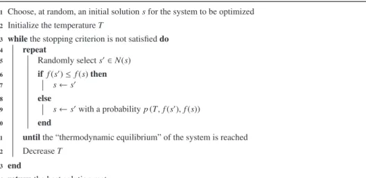
The algorithm starts by generating an initial solution (either randomly or constructed using an heuristic) and by initial- izing the temperature paramete rT. Then, at each iteration, a solution s⁰is randomly selected in the neighborho od N(s) of the current solution s. The solution s⁰is accepted as new current solution depending on Tand on the values of the objective function for s⁰ands, denoted by f(s⁰) and f(s), respectively. If f(s⁰)6f(s), then s⁰is accepted and it replaces s. On the other hand, if f(s⁰) >f(s),s⁰can also be accepted, with a probability pðT;fðs⁰Þ;fðsÞÞ ¼exp^fðs⁰^Þf_T ^ðsÞ

. The temperature Tis decrease d during the search process, thus at the beginning of the search, the probability of accepting deteriorati ng moves is high and it grad- ually decreases. The high level SA algorithm is presented in Fig. 1.

(3)

One can notice that the algorithm can converge to a solution s, even if a better solution s⁰is met during the search process.

Then, a basic improvement of SA consists in saving the best solution met during the search process.

SA has been successfully applied to several discrete or continuous optimization problems, though it has been found too greedy or unable to solve some combinatori al problems. The adaptation of SA to continuous optimization problems has been particularly studied [58]. A wide bibliography can be found in [57,90,152,157,25 5,259] .

Several variants of SA have been proposed in the literature. Three of them are described below.

2.1.1. Microcanonic annealing

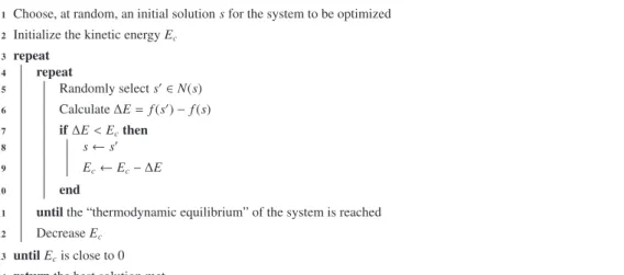
The principle of Microcanon ic Annealing (MA) is similar to that of SA, and MA can be considered as a variant of SA. The main differenc e is that instead of using a Metropolis algorithm, MA uses the Creutz algorithm [59], known as microcanoni cal Monte Carlo simulatio n or ‘‘demon’’ algorithm. The Creutz algorithm allows reaching the thermodyna mic equilibriu m in an isolated system, i.e. a system where the total energy, which is the sum of the potential energy and the kinetic energy, remains constant (Etotal=Ep+Ec).

For an optimization problem, the potential energy Epcan be considered as the objective function, to be minimized. The kinetic energy Ecis used in a similar manner to the temperature in simulated annealing; it is forced to remain positive. The algorithm accepts all disturbance s which cause moves towards the lower energy states, by adding DE(lost potential energy) to the kinetic energy Ec. The moves towards higher energy states are only accepted when DE<Ec, and the energy acquired in the form of potential energy is cut off from the kinetic energy. Thus, the total energy remains constant. The MA algorithm is presented in Fig. 2.

At each energy stage, the ‘‘thermodynam ic equilibrium ’’ is reached as soon as the ratio req¼_r^hE_ðE^c_cⁱ_Þof the average kinetic energy observed to the standard deviation of the distribution of Ecis ‘‘close’’ to 1.

Eq.(1)involving the kinetic energy and the temperat ure establishes a link between SA and MA, where kBdenotes the Boltzmann constant.

kBT¼ hEci ð1Þ

MA has several advantag es compared to simulated annealing. It neither requires the transcendent functions like expto be evaluated, nor any random number to be drawn for the acceptance or the rejection of a solution. Their computations can be indeed time costly. A relatively recent work shows the successfu l applicati on of MA, hybridized with the Nelder-M ead simplex method [193], in microscopic image processin g[191].

2.1.2. Threshold accepting method

Another variant of SA is the Threshold Accepting method (TA)[77]. The principal difference between TA and SA lies in the criterion for acceptance of the candidate solutions: on the one hand, SA accepts a solution that causes deterioration of the objective function fonly with a certain probability; on the other hand, TA accepts this solution if the degradation of fdoes not exceed a progressive ly decreasing threshold T. The TA algorithm is presented in Fig. 3.

The TA method compares favorably with simulated annealing for combinatori al optimizati on problems , like the traveling salesman problem [76]. An adaptation of TA to continuous optimization can be carried out similarly to SA.

Fig. 1. Algorithm for the simulated annealing method.

(4)

2.1.3. Noising method

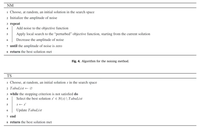
The Noising Method (NM) was proposed by Charon and Hudry [45]. Initially proposed for the clique partitioni ng problem in a graph, it has been shown to be successful for many combinatori al optimizati on problems. It uses a local search algorithm, i.e. an algorithm which, starting from an initial solution, carries out iterative improvements until obtaining a local optimum.

The basic idea of NM is as follows. Rather than taking the genuine data of an optimization problem directly into account, the data are ‘‘perturb ed’’, i.e. the values taken by the objective function are modiﬁed in a certain way. Then, the local search algorithm is applied to the perturbed function. At each iteration of NM, the amplitude of the noising of the objective function decreases until it is zero. The reason behind the addition of noise is to be able to escape any possible local optimum of the objective function. In NM, a noise is a value taken by a random variable following a given probability distribution (e.g. uniform or Gaussian law). The algorithm for NM is presented in Fig. 4.

The authors proposed and analysed different ways to add noise [46]. They showed that, accordin g to the noising carried out, NM can be made identical with SA, or with TA, described above. Thus, NM represents a generalization of SA and TA. They also published a survey in [47], and recently, they proposed a way to design NM that can tune its paramete rs itself [48].

2.2. Tabu search

Tabu Search (TS) was formalized in 1986 by Glover [104]. TS was designed to manage an embedded local search algorithm. It explicitly uses the history of the search, both to escape from local minima and to implement an explorative strategy.

Its main characterist ic is indeed based on the use of mechanis ms inspired by the human memory. It takes, from this point of view, a path opposite to that of SA, which does not use memory, and thus is unable to learn from the past.

Fig. 3. Algorithm for the threshold accepting method.

Fig. 2. Algorithm for the microcanonic annealing method.

(5)

Various types of memory structures are commonly used to remember speciﬁc properties of the trajectory through the search space that the algorithm has undertak en. Atabu list (from which the name of the metaheu ristic framework derives) records the last encountered solutions (or some attributes of them) and forbids these solutions (or solutions containing one of these attributes ) from being visited again, as long as they are in the list. This list can be viewed as short-term memory, that records information on recently visited solutions. Its use prevents from returning to recently visited solutions, therefore it prevents from endless cycling and forces the search to accept even deteriorating moves. A simple TS algorithm is presented inFig. 5.

The length of the tabu list controls the memory of the search process. If the length of the list is low, the search will con- centrate on small areas of the search space. On the opposite, a high length forces the search process to explore larger regions, because it forbids revisiting a higher number of solutions. This length can be varied during the search, leading to more robust algorithms, like the Reactive Tabu Search algorithm [19].

Additional intermedi ate-term memory structures can be introduced to bias moves towards promising areas of the search space (intensiﬁcation), as well as long-term memory structure s to encourag e broader exploration of the search space (diversiﬁcation).

The addition of intermediate- term memory structure s, called aspiration criteria , can greatly improve the search process.

Indeed, the use of a tabu list can prevent attractive moves, even if there is no risk of cycling, or they may lead to an overall stagnation of the search process. For example, a move which leads to a solution better than all those visited by the search in the preceding iterations does not have any reason to be prohibited. Then, the aspiration criteria, that are a set of rules, are used to override tabu restrictions, i.e. if a move is forbidden by the tabu list, then the aspiratio n criteria, if satisﬁed, can allow this move.

A frequency memory can also be used as a type of long-term memory. This memory structure records how often certain attributes have been encountered in solutions on the search trajector y, which allows the search to avoid visiting solutions that present the most often encountered attributes or to visit solutions with attributes rarely encountered.

An extensive description of TS and its concepts can be found in [107]. Good reviews of the method are provided in [100,101]. TS was designed for, and has predominatel y been applied to combinatorial optimizati on problems . However, adaptations of TS to continuous optimization problems have been proposed [105,60,49].

2.3. GRASP method

GRASP, for Greedy Randomiz ed Adaptive Search Procedure , is a memory-less multi-sta rt metaheurist ic for combinatori al optimization problems, proposed by Feo and Resende in [84,85]. Each iteration of the GRASP algorithm consists of two

Fig. 4. Algorithm for the noising method.

Fig. 5. Algorithm for the simple tabu search method.

(6)

steps: construction and local search. The construction step of GRASP is similar to the semi-greedy heuristic proposed inde- pendently by Hart and Shogan [129]. The construction step builds a feasible solution using a randomized greedy heuristic.

In the second step, this solution is used as the initial solution of a local search procedure. After a given number of iterations, the GRASP algorithm terminat es and the best solution found is returned. A template for the GRASP algorithm is presented in Fig. 6.

In the greedy heuristic, a candidate solution is built iteratively, i.e. at each iteration, an element is incorporated into a partial solution, until a complete solution is built. It means that, for a given problem, one has to define a solution as a set of elements . At each iteration of the heuristic, the list of candidate elements is formed by all the elements that can be included in the partial solution, without destroying feasibility. This list is ordered with respect to a greedy function, that mea- sures the benefit of selecting each element. Then, the element to be added to the partial solution is randomly chosen among the best candidates in this list. The list of the best candidates is called the restricted candidate list (RCL). This random selection of an element in the RCL represents the probabili stic aspect of GRASP. The RCL list can be limited either by the number of elements (cardinality-based) or by their quality (value-based). In the first case, the RCL list consists of the pbest candidate elements, where pis a parameter of the algorithm. In the second case, it consists of the candidate elements having an incre- mental cost (the value of the greedy function) greater or equal to c^min+

a

(c^max c^min), where

a

is a paramete r of the algorithm, and c^minandc^maxare the values of the best and worst elements, respectively. This is the most used strategy [221], and

a

is the main paramete r of GRASP, where

a

2[0, 1]. Indeed, this parameter defines the compromise between intensification and diversification.

The performance of GRASP is very sensitive to the

a

parameter, and many strategies have been proposed to ﬁt it [258]

(initialized to a constant value, dynamically changed according to some probability distribution , or automatically adapted during the search process). A self-tuning of

a

is performed in reactive GRASP , where the value of

a

is periodically updated according to the quality of the obtained solutions [214].

Festa and Resende surveyed the algorithmic aspects of GRASP [86], and its applicati on to combinatori al optimization problems[87]. A good bibliograp hy is provided also in [222]. GRASP can be hybridize d in different ways, for instance by replacing the local search with another metaheurist ic such as tabu search, simulated annealing, variable neighborho od search, iterated local search, among others [220,271,23 5] . It is also often combined with a path-reli nking strategy [88]. Adap- tations to continuous optimization problems have also been proposed [134].

2.4. Variable neighborho od search

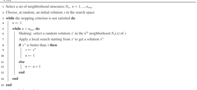
Variable Neighborhood Search (VNS) is a metaheuristic proposed by Hansen and Mladenovic [184,186]. Its strategy consists in the exploration of dynamically changing neighborhoods for a given solution. At the initializatio n step, a set of neighborhood structure s has to be deﬁned. These neighborho ods can be arbitrarily chosen, but often a sequence N1;N2;. . .;Nnmaxof neighborho ods with increasing cardinality is deﬁned. In principle they could be included one in the other

(N12N22. . .2Nnmax). However, such a sequence may produce an inefﬁcient search, because a large number of solutions

can be revisited [33]. Then an initial solution is generated, and the main cycle of VNS begins. This cycle consists of three steps:shaking,local search andmove. In the shaking step, a solution s⁰ is randomly selected in the nth neighborho od of the current solution s. Then, s⁰is used as the initial solution of a local search procedure, to generate the solution s⁰⁰. The local search can use any neighborho od structure and is not restricted to the set Nn,n= 1, . . .,nmax. At the end of the local search process, if s⁰⁰is better than s, then s⁰⁰replacessand the cycle starts again with n= 1. Otherwise, the algorithm moves to the next neighborho od n+ 1 and a new shaking phase starts using this neighborhood. The VNS algorithm is presente d in Fig. 7.

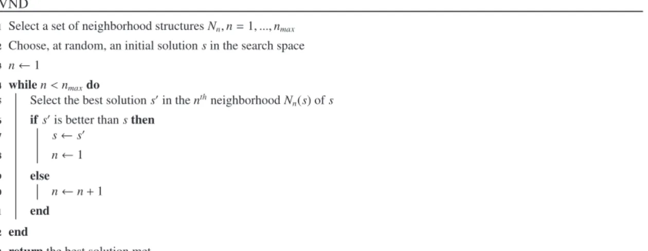
This algorithm is efﬁcient if the neighborho ods used are complemen tary, i.e. if a local optimum for a neighborho od Niis not a local optimum for a neighborhood Nj. VNS is based on the variable neighborho od descent (VND), which is a deterministic version of VNS [258]described in Fig. 8. A more general VNS algorithm (GVNS), where VND is used as the local search procedure of VNS, has led to many successfu l applications [122]. Recent surveys of VNS and its extensions are available in [122,123]. Adaptations to continuous optimization problems have been proposed in [164,185 ,37] . Hybridization of VNS with other metaheurist ics, such as GRASP, is also common [271,235]. The use of more than one neighborho od structure is not restricted to algorithms labeled VNS [250]. In Reactive Search [18], a sophisticated adaptatio n of the neighborho od is performed, instead of cycling over a predeﬁned set of neighborhoods.

Fig. 6. Template for the GRASP algorithm.

(7)

2.5. Guided local search

As tabu search, Guided Local Search (GLS)[272,274]makes use of a memory. In GLS, this memory is called an augmented objective function . Indeed, GLS dynamically changes the objective function optimized by a local search, according to the found local optima. First, a set of features ftn,n= 1, . . .,nmaxhas to be defined. Each feature defines a characterist ic of a solution regarding the optimization problem to solve. Then, a cost ciand a penalty value piare associate d with each feature. For instance, in the traveling salesman problem, a feature ftican be the presence of an edge from a city A to a city B in the solution, and the corresponding cost cican be the distance, or the travel time, between these two cities. The penalties are initialized to 0 and updated when the local search reaches a local optimum. Given an objective function fand a solution s, GLS defines the augmented objective function f⁰as follows:

f⁰ðsÞ ¼fðsÞ þkXⁿ^max

i¼1

p_iIiðsÞ ð2Þ

wherekis a paramete r of the algorithm, and Ii(s) is an indicator function that determines whether sexhibits the feature fti: IiðsÞ ¼ 1 if sexhibits the feature ft_i

0 otherwise

ð3Þ

Fig. 7. Template for the variable neighborhood search algorithm.

Fig. 8. Template for the variable neighborhood descent algorithm.

(8)

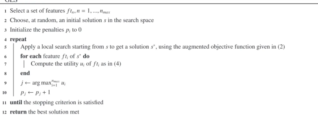
Each time a local optimum is found by the local search, GLS intends to penalize the most ‘‘unfavorabl e features’’ of this local optimum, i.e. the features having a high cost. This way, solutions exhibiting other features become more attractive, and the search can escape from the local optimum. When a local optimum s^⁄is reached, the utility uiof penalizing a feature ftiis calculated as follows:

uðsÞ ¼IiðsÞ ci

1þpi

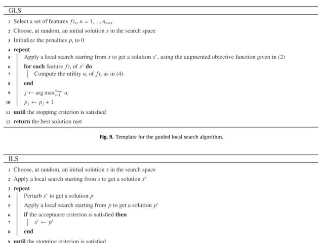
ð4Þ The greater the cost ciof this feature, the greater the utility to penalize it is. Besides, the more times it has been penalized (the greater pi), the lower the utility of penalizing it again is. The feature having the greatest utility value is penalized: its penalty value piis increased by 1. In the augmented objective function, the scaling of the penality is adjusted by k. Authors suggest that the performance of GLS is not very sensitive to the value of k[183]. Large values of kencourage diversiﬁcation, while small values intensify the search around the local optimum [258]. GLS algorithm is summari zed in Fig. 9.

Sitting on top of a local search algorithm, the adaptation of GLS to continuous optimization is straightforwar d[273].

Extensions to population based metaheurist ics have been proposed [160,286,257]. Mills et al. proposed an extended guided local search algorithm (EGLS), adding aspiration criteria and random moves to GLS [182,183]. A recent survey on GLS and its applications is available in [276,275].

2.6. Iterated local search

The deﬁnition and framework of Iterated Local Search (ILS) are given by Stützle in his PhD dissertat ion [254]. Stützle does not take credit for the approach, and instead highlights speciﬁc instances of ILS from the literature, such as iterated descent [20],large-step Markov chains [176],iterated Lin-Kernigha n[139],chained local optimization [175], as well as [21]that introduces the principle, and [140]that summarizes it (list taken from [168,36]).

ILS is a metaheurist ic based on a simple idea: instead of repeatedly applying a local search procedure to randomly generated starting solutions, ILS generates the starting solution for the next iteration by perturbing the local optimum found at

Fig. 9. Template for the guided local search algorithm.

Fig. 10. Template for the iterated local search algorithm.

(9)

the current iteration. This is done in the expectati on that the perturba tion mechanism provides a solution located in the basin of attraction of a better local optimum. The perturbation mechanism is a key feature of ILS: on the one hand, a too weak perturbation may not be sufﬁcient to escape from the basin of attraction of the current local optimum; on the other hand, a too strong perturba tion would make the algorithm similar to a multistart local search with randomly generate d starting solutions. ILS algorithm is summarized in Fig. 10 , where the acceptanc e criterion deﬁnes the conditions that the new local optimump^⁄has to satisfy in order to replace the current one s^⁄.

The acceptance criterion, combined with the perturbation mechanis m, enables controlling the trade-off between intensification and diversification. For instance, an extreme acceptance criterion in terms of intensification is to accept only improving solutions. Another extreme criterion in terms of diversification is to accept any solution, without regard to its quality. Many acceptance criteria that balance the two goals may be applied [258].

A recent review of ILS, its extension s and its applications is available in [168].

3. Population-base d metaheu ristics

Population- based metaheuristics deal with a set (i.e. a population) of solutions rather than with a single solution. The most studied population-based methods are related to Evolutionar y Computation (EC) and Swarm Intelligence (SI). EC algorithms are inspired by Darwin’s evolutionar y theory, where a population of individuals is modiﬁed through recombin ation and mutation operators. In SI, the idea is to produce computati onal intelligence by exploitin g simple analogs of social interaction, rather than purely individual cognitive abilities.

3.1. Evolutionary computation

Evolutionary Computation (EC) is the general term for several optimization algorithms that are inspired by the Darwinian principles of nature’s capability to evolve living beings well adapted to their environment. Usually found grouped under the term of EC algorithms (also called Evolutionary Algorithms (EAs)), are the domains of genetic algorithms [135], evolution strategies[217], evolutionary programmin g [95], and genetic programming [154]. Despite the differences between these techniques, which will be shown later, they all share a commun underlyin g idea of simulating the evolution of individual structures via processes of selection, recombin ation, and mutation reproduction, thereby producing better solutions.

A generic form of a basic EA is shown in Fig. 11 . This form will serve as a template for algorithms that will be discussed throughout this section.

Every iteration of the algorithm corresponds to ageneration, where apopulationof candidate solutions to a given optimization problem, called individuals, is capable of reproducing and is subject to genetic variations followed by the environm en- tal pressure that causes natural selection (survival of the fittest). New solutions are created by applying recombin ation , that combines two or more selected individuals (the so-called parents) to produce one or more new individuals (thechildrenor offspring), and mutation, that allows the appearance of new traits in the offspring to promote diversity. The fitness(how good the solutions are) of the resulting solutions is evaluated and a suitable selection strategy is then applied to determine which solutions will be maintain ed into the next generation. As a termination condition, a predefined number of generations (or function evaluations ) of simulated evolutionary process is usually used, or some more complex stopping criteria can be applied.

Over the years, there have been many overviews and surveys about EAs. The readers interested in the history are referred to[13,10]. EAs have been widely applied with a good measure of success to combinatori al optimization problems [33,26], constrained optimization problems [55], Data Mining and Knowledge Discovery [97], etc. Multi-Objective Evolutionary Algo- rithms (MOEAs) are one of the current trends in developing EAs. An excellent overview of current issues, algorithms, and existing systems in this area is presented in [54]. Parallel EAs have also deserved interest in the recent past (a good review

Fig. 11. Evolutionary computation algorithm.

(10)

can be found in [5]). Another overview paper over self-adaptiv e methods in EAs is given in [180]. They are called self-adaptive, because these algorithms control the setting of their parameters themselves, embedding them into an individua l’s gen- ome and evolving them. Some other topics covered by the literature include the use of hybrid EAs, that combine local search or some other heuristic search methods [32].

3.1.1. Genetic algorithm

The Genetic Algorithm (GA) is arguably the most well-known and mostly used evolutionary computation technique. It was originally develope d in the early 1970s at the University of Michigan by John Holland and his students, whose research interests were devoted to the study of adaptive systems [135]. The basic GA is very generic, and there are many aspects that can be impleme nted differently according to the problem: representat ion of solution (chromosomes), selection strategy, type of crossover (the recombination operator of GAs) and mutation operators, etc. The most common represen- tation of the chromosomes applied in GAs is a fixed-lengthbinarystring. Simple bit manipulation operations allow the implementati on of crossoverandmutationoperation s. These genetic operators form the essential part of the GA as a problem-solving strategy. Emphasis is mainly concentrated on crossove r as the main variation operator, that combines multiple (usually two) individuals that have been selected together by exchanging some of their parts. There are various strategies to do this, e.g. n-pointanduniform crossover . An exogenous parameter p_c(crossover rate ) indicates the probability per individual to undergo crossover. Typical values for pcare in the range [0.6,1.0] [13]. Individuals for producing offspring are chosen using a selection strategy after evaluating the fitness value of each individual in the selection pool. Some of the popular selection schemes are roulette-whe el selection ,tournament selection ,ranking selection , etc. A comparison of selection schemes used in GAs is given in [111,30]. After crossove r, individuals are subjected to mutation. Mutation introduces some randomness into the search to prevent the optimization process from getting trapped into local optima. It is usually considered as a secondar y genetic operator that performs a slight perturba tion to the resulting solutions with some low prob- abilitypm. Typically, the mutation rate is applied with less than 1% probability, but the appropriate value of the mutation rate for a given optimization problem is an open research issue. The replacement(survivor selection ) uses the fitness value to identify the individuals to maintain as parents for successive generations and is responsible to assure the survival of the fittest individuals. Interested readers may consult the book by Goldberg [110]for more detailed background information on GAs.

Since then, many variants of GAs have been developed and applied to a wide range of optimization problems. Overviews concerning current issues on GAs can be found in [22,23],[249]for hybrid GAs, [151]for multi-obj ective optimization and [6]for Parallel GAs, among others. Indexed bibliographi es of GAs have been compiled by Jarmo T. Alander in various application areas, like in robotics, Software Engineering, Optics and Image Processing, etc. Versions of these bibliographi es are available via anonymous ftporwwwfrom the following site: ftp.uwasa. fi/cs/rep ort94–1.

3.1.2. Evolution Strategy

Similar to GA, Evolution Strategy (ES) imitates the principles of natural evolution as a method to solve optimizati on problems. It was introduced in the 60ies by Rechenberg [216,217]and further developed by Schwefel. The first ES algorithm, used in the field of experime ntal parameter optimization, was a simple mutation-se lection scheme called two membered ES . Such ES is based upon a population consisting of a single parent which produces, by means of normally (Gaussian) distributed mutation, a single descendant. The selection operator then determines the fitter individual to become the parent of the next generation.

To introduce the concept of population, which has not really been used so far, Rechenbe rg proposed the multimembered ES, where

l

> 1 parents can participate in the generation of one offspring individua l. This has been denoted by (

l

+ 1)ES.

With the introduct ion of more than one parent, an additional recombin ation operator is possible. Two of the

l

parents are chosen at random and recombin ed to give life to an offspring, which also underlies mutation. The selection resembles

‘‘extinction of the worst’’, may it be the offspring or one of the parents, thus keeping constant the population size. Schwefel [237]introduced two further versions of multimembered ES , i.e. (

l

+k)ES and (

l

,k)ES. The ﬁrst case indicates that

l

parents create kP1 descenda nts by means of recombination and mutation, and, to keep the population size constant , the k worst out of all

l

+ kindividuals are discarded. For a (

l

,k)ES, with k>

l

, the

l

best individuals of the koffspring become the parents of the next population, whereas their parents are deleted, no matter how good or bad their ﬁtness was compared to that of the new generation’s individuals. Two other well-known ES versions are known as (

l

/

q

+k)ES and (

l

/

q

,k)ES).

The additional paramete r

q

refers to the number of parents involved in the procreation of one offspring.

The mutation in ES is realized through normally distributed numbers with zero mean and standard deviation

r

, which can be interpreted as the mutation step size . It is easy to imagine that the parameters of the normal distribution play an essential role for the performanc e of the search algorithm. The simplest method to specify the mutation mechanism is to keep

r

constant over time. Another approach consists in dynamically adjusting

r

by assigning different values depending on the number of generations or by incorporating feedback from the search process. Various methods to control the mutation paramete r have been developed. Among these there are for example Rechenberg ’s 1/5 success rule ¹ [217], the

1The 1/5 rule in (1 + 1)ES states that: the ratio of successful mutations to all mutations should be 1/5. If it is greater than 1/5, increase the variance; if it is less, decrease the mutation variance .

(11)

r

-self-adap tation (

r

SA)²[217], the meta-ES (mES)³[239], a hierar chically organized population based ES involving isolation periods[132], the mutative self adaptat ion [238], the machine learning approache s[240], or the cumulative pathlength control [197].

Adaptivity is not limited to a single paramete r, like the step-size. More recently, a surprisingly effective method, called the Covariance Matrix Adaptation Evolution Strategy (CMA-ES), was introduced by Hansen, Ostermeier, and Gawelczyk [121]and further developed in [120]. The CMA-ES is currently the most widely used, and it turns out to be a particularly reliable and highly competitive EA for local optimization [120]and also for global optimization [119]. In the ‘‘Special Session on Real- Parameter Optimizatio n’’ held at the CEC 2005 Congress, the CMA-ES algorithm obtained the best results among all the evaluated techniques on a benchmark of 25 continuous functions [9]. The performances of the CMA-ES algorithm are also compared to those of other approaches in the Workshop on Black-Box Optimization Benchmarking BBOB’200 9 and on the test functions of the BBOB’2010.

In recent years, a fair amount of theoretical investigation has contributed substantially to the understand ing of the evolutionary search strategies on a variety of problem classes. A number of review papers and text books exist with such details to which the reader is referred (see[11,13,25,156]).

3.1.3. Evolutionary programmi ng

Evolutionary Programmi ng (EP) was ﬁrst presented in the 1960s by L.J. Fogel as an evolutionary approach to artiﬁcial intelligence[95]. Later, in the early 1990s, EP was reintroduce d by D. Fogel to solve more general tasks including prediction problems, numerical and combinatori al optimization, and machine learning [91,92].

The representat ions used in EP are typically tailored to the problem domain. In real-valued vector optimizati on, the cod- ing will be taken naturally as a string of real values. The initial population is selected at random with respect to a density function and is scored with respect to the given objective. In contrast to the GAs, the conventi onal EP does not rely on any kind of recombinati on. The mutation is the only operator used to generate new offspring. It is impleme nted by adding a random number of certain distribution s to the parent. In the case of standard EP, the normally distributed random mutation is applied. However , other mutation schemes have been proposed. D. Fogel [93]developed an extension of the standard EP, called meta-EP, that self-adapts the standard deviations (or equivalently the variances). The R-meta-EPalgorithm[94]

incorporate s the self-adaptation of covariance matrices in addition to standard deviations. Yao and Liu [284]substituted the normal distribution of the meta-EPoperator with a Cauchy-distr ibution in their new algorithm, called fast evolution ary programmin g(FEP). In [162], Lee and Yao proposed to use a Levy-distributi on for higher variation s and a greater diversity. In Yao’sImproved Fast Evolutionary Programming algorithm (IFEP)[285], two offspring are created from each parent, one using a Gaussian distribution, and the other using the Cauchy distribution . The parent selection mechanism is deterministic. The survivor selection process (replacement) is probabilistic and is based on a stochastic tournament selection. The framework of EP is less used than the other families of EAs, due to its similarity with ES, as it turned out in [12].

3.1.4. Genetic programming

The Genetic Programmi ng (GP) became a popular search technique in the early 1990s due to the work by Koza [154]. It is an automate d method for creating a working computer program from a high-level problem statement of ‘‘ what needs to be done’’.

GP adopts a similar search strategy as a GA, but uses a program representat ion and special operators. In GP, the individua l population members are not ﬁxed-length strings as used in GAs, they are computer programs that, when executed, are the candidate solutions to the problem at hand. These programs are usually expresse d as syntax trees rather than as lines of code, which provides a ﬂexible way of describing them in LISP language, as originally used by J. Koza. The variables and constants in the program, called terminalsin GP, are leaves of the tree, while the arithmetic operations are internal nodes (typically calledfunctions). The terminal and function sets form the alphabets of the programs to be made.

GP starts with an initial population of randomly generated computer programs compose d of functions and terminals appropriate to the problem domain. There are many ways to generate the initial population resulting in initial random trees of different sizes and shapes. Two of the basic ways, used in most GP systems are called fullandgrowmethods. The fullmeth- od creates trees for which the length of every nonbacktrac king path between an endpoint and the root is equal to the specified maximum depth. ⁴Thegrowmethod involves growing trees that are variably shaped. The length of a path between an endpoint and the root is no greater than the specified maximum depth. A widely used combin ation of the two methods, known asRamped half-and-h alf [154], involves creating an equal number of trees using a depth parameter that ranges between 2 and the maximum specified depth. While these methods are easy to implement and use, they often make it difficult to control the statistical distribu tions of important properties such as the sizes and shapes of the generated trees [280]. Other initializatio n mechan isms, however, have been developed to create different distributions of initial trees, where the general consensus is that a more uniform and random distribu tion is better for the evolution ary process [170].

2 Instead of changing rby an exogenous heuristic in a determin istic manner, Schwefel completely viewed ras a part of genetic information of an individual, which can be interpreted as self-adapta tion of step sizes . Consequently, it is subject to recombination and mutation as well.

3 rSA and mES do not exclude each other. A mES may perform SA and a SA can include a lifetime mechanism allowing a variable lifespan of certain individuals.

4 The depth of a tree is deﬁned as the length of the longest nonbacktracking path from the root to an endpoint.

(12)

The population of programs is then progressive ly evolved over a series of generations , using the principles of Darwinian natural selection and biologically inspired operations, including crossover and mutation, which are specialized to act on computer programs. To create the next population of individuals, computer programs are probabili stically selected, in pro- portion to fitness, from the current population of programs. That is, better individuals are more likely to have more child programs than inferior individuals. The most commonly employed method for selecting individuals in GP is tournament selection, followed by fitness-proportionate selection , but any standard EA selection mechanism can be used [209]. Recombi- nation is usually implemented as subtree crossover between two parents. The resulting offspring are composed of subtrees from their parents that may be of different sizes and in different positions in their programs. Other forms of crossover have been defined and used, such as one-point crossover ,context-preserv ing crossover ,size-fair crossover anduniform crossover [209]. Mutation is another important feature of GP. The most commonly used form of mutation is subtree mutation , which randomly selects a mutation point in a tree and substitutes the subtree rooted there with a randomly generated subtree.

Other forms of mutation include single-node mutations and various forms of code-editing to remove unnecessar y code from trees have been proposed in the literature [209,206]. Also, often, in addition to crossove r and mutation, an operation which simply copies selected individuals in the next generation is used. This operation , called reproduct ion , is typically applied only to produce a fraction of the new generation [280]. The replacementphase concerns the survivor selection of both parent and offspring populations. There are two alternatives for implementing this step: the generationalapproach, where the offspring population will replace systematical ly the parent population and the steady-stateapproach, where the parent population is maintained and some of its individuals are replaced by new individuals according to some rules. Advanced GP issues concern developingautomatical ly deﬁned functions and specialized operators, such as permutation,editing, or encapsulation[155].

The theoretical foundations of GP as well as a review of many real-world applications and important extensions of GP are given in [209,280,177]. Contemporar y GPs are widely used in machine learning and data mining tasks, such as prediction and classiﬁcation. There is also a great amount of work done on GP using probabilistic models. The intereste d reader should refer to[243]which is a review that includes directions for further research on this area.

3.2. Other evolutionary algorithm s

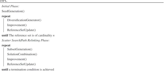
Other models of evolutionary algorithms have been proposed in the literature. Among them, one can ﬁnd estimation of distribution algorithms, differential evolution, coevolution ary algorithms, cultural algorithms and Scatter Search and Path Relinking.

3.2.1. Estimation of distribution algorithms

Estimation of Distribution Algorithms (EDAs), also referred to as Probabilistic Model-Buildin g Genetic Algorithm s (PMBGA), were introduced in the ﬁeld of evolutionary computation, for the ﬁrst time, by Mühlenbein and Paaß[190]. These algorithms are based on probabili stic models, where genetic recombination and mutation operator s of GA are replaced by the following two steps: (1) estimate the probabili ty distribution of selected individua ls (promising solutions) and (2) generate new population by sampling this probability distribution . This leads the search towards promising areas of the space of solutions. The new solutions are then incorporated into the original population, replacing some of the old ones or all of them.

The process is repeated until the terminat ion criteria are met. The type of probabilistic models used by EDAs and the methods employed to learn them may vary according to the characteristics of the optimizati on problem.

Based on this general framewor k, several EDA approaches have been develope d in the last years, where each approach learns a speciﬁc probabilistic model that conditions the behavior of the EDA from the point of view of complexity and performance. EDAs can be broadly divided into three classes, according to the complexity of the probabilistic models used to capture the interdependen cies between the variables: starting with methods that assume total independency between problem variables (univariateEDAs), through the ones that take into account some pairwise interactions (bivariateEDAs), to the methods that can accurately model even a very complex problem structure with highly overlapping multivariate building blocks (multivari ate EDAs)[159].

In all the approach es belonging to the ﬁrst category, it is assumed that the n-dimensional joint probability distribution of solutions can be factored as a product of independen t univariat e probability distribut ions. Algorithms based on this principle work very well on linear problems where the variables are not mutually interacting [188]. It must be noted that, in difﬁcult optimization problems, different dependency relations can appear between variables and, hence, considering all of them independen t may provide a model that does not represent the problem accurately. Common univariateEDAs include Popu- lation Based Incrementa l Learning (PBIL)[14], Univariate Marginal Distribut ion Algorithm (UMDA)[188]and Compact Ge- netic Algorithm (cGA)[125].

In contrast to univariat e EDAs, algorithms in the bivariateEDAs category consider dependenci es between pairs of variables. In this case, it is enough to consider second-order statistics. Examples of such algorithms are Mutual Informati on Max- imizing Input Clustering algorithm (MIMIC)[66], Combining Optimizers with Mutual Information Trees (COMIT)[15]and Bivariate Marginal Distribution Algorithm (BMDA) [205]. These algorithms reproduce and mix building blocks of order two very efﬁciently, and therefore they work very well on linear and quadratic problems . Nonetheless, capturing only some pair-wise interactions has still shown to be insufﬁcient for solving problems with multivariate or highly overlapping building blocks. That is why multivariateEDAs algorithms have been proposed.

(13)

Algorithms belonging to this last category use statistics of order greater than two to factorize the probabili ty distribution.

In this way, multivariate interactio ns between problem variables can be expressed properly without any kind of initial restriction. The best known multivari ate EDAs are Bayesian Optimizatio n Algorithm (BOA)[202,203], Estimation of Bayesian Networks Algorithm (EBNA)[82], Factorized Distribution Algorithm (FDA) [189], Extended Compact Genetic Algorithm (EcGA)[124]and Polytree Approximati on Distribution Algorithm (PADA)[251]. Those EDAs that look for multi-depen dencies are capable of solving many hard problems accurately, and reliably with the sacrifice of computation time due to the complexity of the learning interactions among variables. Nonetheless , despite increased computati onal time, the number of evaluations of the optimized function is reduced significantly. That is why the overall time complexity is significantly reduced for large problems [204].

EDAs have been applied to a variety of problems in domains such as engineeri ng, biomedical informatics, and robotics. A detailed overview of different EDA approach es in both discrete and continuo us domains can be found in [159]and a recent survey was published in [130]. However , despite their successful applicati on, there are a wide variety of open questions [236]regarding the behavior of this type of algorithms.

3.2.2. Differential evolution

Differential Evolution (DE) algorithm is one of the most popular algorithm for the continuo us global optimization problems. It was proposed by Storn and Price in the 90’s [253]in order to solve the Chebyshev polynomial ﬁtting problem and has proven to be a very reliable optimizati on strategy for many different tasks.

Like any evolutionary algorithm, a population of candidate solutions for the optimizati on task to be solved is arbitrarily initialized. For each generation of the evolution process, new individuals are created by applying reproduction operator s (crossover and mutation). The ﬁtness of the resulting solutions is evaluated and each individua l (target individual ) of the population competes against a new individual (trial individual ) to determine which one will be maintained into the next generation. The trial individual is created by recombinin g the target individua l with another individual created by mutation (called mutant individual ). Different variants of DE have been suggested by Price et al. [215]and are conventional ly named DE/ x/ y/ z, whereDEstands for Differential Evolution, xrepresents a string that denotes the base vector, i.e. the vector being perturbed, whether it is ‘‘ rand’’ (a randomly selected population vector) or ‘‘ best’’ (the best vector in the population with respect to ﬁt- ness value),yis the number of difference vectors considered for perturbation of the base vector xandzdenotes the crossover scheme, which may be binomialorexponential. The DE/rand/1/bi n-variant, also known as the classical version of DE, is used later on for the description of the DE algorithm.

The mutation in DE is performed by calculatin g vector differences between other randomly selected individua ls of the same population. There are several variants how to generate the mutant individual . The most frequently used mutation strategy (calledDE/rand/1/bi n) generates the trial vector V!

i;gby adding only one weighted difference vector FðX!

r2;g!X

r3;gÞto a randomly selected base vector !X

r1;gto perturb it. Speciﬁcally, for each target vector !X

i;g,i= 1, 2, . . .,N, where gdenotes the current generation and Nthe number of individua ls in the population, a mutant vector is produced using the following formula:

!V

i;g¼!X

r₁;gþFð!X

r₂;g!X

r₃;gÞ ð5Þ

where the indexes r1,r2andr3are randomly chosen over [1, N] and should be mutually different from the running index i.Fis a real constant scaling factor within the range [0, 1].

Based on the mutant vector, a trial vector U!

i;gis constructed through a crossover operation which combines components from the ith population vector !X

i;gand its corresponding mutant vector V!

i;g: Ui;j;g¼ Vi;j;g ifrandð0;1Þ6CRorj¼jrand

Xi;j;g otherwise

ð6Þ The crossover factor CRis randomly taken from the interval [0, 1] and presents the probability of creating parameters for trial vector from a mutant vector. Index j_randis a randomly chosen integer within the range [1, N]. It is responsible for the trial vector containing at least one parameter from the mutant vector. rand(0, 1) is a uniform random number in range [0, 1].

j= 1, 2, . . .,D, where Dis the number of paramete rs (dimension) of a single vector.

Finally, to decide whether or not it should become a member of generation g+ 1, the trial vector U!

i;gis compared to the target vector X!

i;gusing the ﬁtness function evaluation:

!X

i;gþ1¼ !U

i;g if fð!U

i;gÞ<fðX!

i;gÞ

!X

i;g otherwise (

ð7Þ The main advantage of the differential evolution consists in its fewer control parameters. It has only three input parameters controlling the search process, namely the population size N, the constant of different iation F, which controls the amplification of the differential variation, and the crossove r control parameter CR. In the original DE, the control parameters are kept fixed during the optimization process. It is not obvious to definea priori which parameter setting should be used as this task is problem specific. Therefore, some researchers (see for example [166,261,35]) have developed various strategie s to make the setting of the paramete rs self-adaptive accordin g to the learning experience.

(14)

DE is currently one of the most popular heuristics to solve single-obj ective optimization problems in continuous search spaces. Due to this success, its use has been extended to other types of problems, such as multi-objective optimization [181].

However, DE has certain ﬂaws, like slow convergence and stagnation of population. Several modiﬁed versions of DE are available in literature for improvin g the performance of basic DE. One class of such algorithms includes hybridized versions, where DE is combined with some other algorithm to produce a new algorithm. For a more detailed description of many of the existing variants and major application areas of DE, readers should refer to [43,194,63].

3.2.3. Coevoluti onary algorithms

When organisms that are ecologically intimate – for example, predators and prey, hosts and parasites, or insects and the ﬂowers that they pollinate – inﬂuence each other’s evolution, we say that coevolutionis occurring. Biologica l coevolution encountered in many natural processes has been an inspiration for coevolutionary algorithms (CoEA), where two or more populations of individuals, each adapting to changes in the other, constantly interact and co-evolve simultaneou sly in contrast with traditional single population EAs.

Signiﬁcant researching into the CoEAs began in the early 1990’s with the seminal work of Hillis [133]on sorting networks.

Contrary to conventional EAs, in which individuals are evaluated independen tly of one another through an absolute ﬁtness measure, the individual ﬁtness in CoEAs is subjective, in the sense that it is a function of its interactions with other individuals.

Many variants of CoEAs have been impleme nted since the beginning of 1990s. These variants fall into two categories:

competitive coevolution andcooperative coevolution . In the case of competitiveapproach es, the different populations compete in solving the global problem and individua ls are rewarded at the expense of those with which they interact. In the case of cooperativeapproaches, however , the various isolated populations are coevolve d to cooperativel y solve the problem; therefore individuals are rewarded when they work well with other individuals and punished when they perform poorly together.

Competitive coevolut ion is usually used to simulate the behavior of competin g forces in nature, such as predators and prey where there is a strong evolutionary pressure for prey to defend themselves better, as future generations of predators develop better attacking strategies. Competitive coevolution can lead to an arms race , in which the two populations have opposing interests and the success of one population depends on the failure of the other. The idea is that continued minor adaptations in some individuals will force competit ive adaptations in others, and these reciprocal forces will drive the algorithms to generate individuals with ever increased performanc e. Individual fitness is evaluated through competition with other individuals in the population. In other words, fitness signifies only the relative strengths of solutions; an increased fitness for one solution leads to a decrease d fitness for another. This inverse fitness interactio n will increase the capabiliti es of each population until the global optimal solution is attained [252]. Competitive coevolution ary models are especially suitable for problem domains where it is difficult to explicitly formulate an objective fitness function. The classic example of competitive coevolution is [133], which coevolved a population of sorting networks . Competitive coevolution has been since successfully applied to game playing strategies [231,210], evolving better pattern recognizers [153], coevolve complex agent behaviors[248], etc.

Cooperative Coevolution is inspired by the ecological relationship of symbiosis where different species live together in a mutually beneficial relationship. A general framework for cooperative coevolut ionary algorithms has been introduced by Potter and De Jong [213]in 1994 for evolving solutions in the form of co-adapted subcomponent s. Potter’s model is usually applied in situations where a complex problem can be decomposed into a collection of easier sub-probl ems. ⁵ Each sub- problem is assigned to a population, such that individual s in a given population represen t potential component s of a larger solution. Evolution of these populations occurs almost simultan eously, but in isolation to one anothe r, interactin g only to obtain fitness. Such a process can be static, in the sense that the division s for the separate componen ts are decided a priori and never altered, or dynamic, in the sense that populations of component s may be added or removed as the run progress es [279]. This model has been analyzed from the evolutionary dynami cs perspecti ve in [171,279]. Cooperative CoEAs have had success in adversaria l domains , e.g., designing artificial neural netwo rks [212], multiobjec tive optimiza tion [260], interaction frequency [211], etc. Some variants of Cooperati ve CoEAs have been propos ed, such as co-evolutionar y particle swarms [131]and coevolutionary differential evolution [246]. A combination of compet itive and cooperative mechanisms has been proposed by Goh et al. [109]to solve multiobjec tive optimiza tion problems in a dynamic environm ent.

Further, both styles of coevolution (i.e., competitive and cooperati ve) can use multiple, reproducti vely isolated populations; both can use similar patterns of inter-pop ulation interaction, similar diversity maintenanc e schemes, and so on. Aside from the novel problem-de composition scheme of cooperative coevolution , the most salient difference between cooperative and competit ive coevolution resides primarily in the game-theor etic properties of the domains to which these algorithms are applied[89].

3.2.4. Cultural algorithm s

Cultural Algorithms (CA) are a class of computational models derived from observing the cultural evolution process in nature[225]. The term culturewas ﬁrst introduced by the anthropologi st Edward B. Taylor in his book, Primitive Culture

5Problem decompo sition consists in determining an appropriate number of subcomponents and the role each will play. The mechanism of dividing the optimization proble mfintonsub-problems and treating them almost independe ntly of one another strongly depends on propert ies of the function f.

(15)

[266]. Taylor offered a broad deﬁnition, stating that culture is ‘‘ that complex whole which includes knowledge, belief, art, morals, law, custom, and any other capabilities and habits acquired by man as a member of society ’’.

The term cultural evolution has been more recently used to refer to the idea that the processes producing cultural stability and change are analogous in important respects to those of biological evolution. In this view, just as biological evolution is characterized by changing frequencies of genes in populations through time as a result of such processes as natural selection, so cultural evolution refers to the changing distribution s of cultural attributes in populations, likewise affected by processes such as natural selection but also by others that have no analog in genetic evolution. Using this idea, Reynolds developed a computational model in which cultural evolution is seen as an inheritance process that operates at both amicro-evoluti onary level in terms of transmission of genetic material between individua ls in a population and amacro-evoluti onary level in terms of the knowled ge acquired based upon individua l experiences. Fundamental of the macro-ev olutionary level is Ren- frew’s notion of individual’s mental mappa, a cognitive map or worldview, that is based on experience with the external world and shapes interactions with it [218]. Individual mappa can be merged and modiﬁed to form group mappa in order to direct the future actions of the group and its individuals.

CAs consist of three components: (1) APopulation Space , at the micro-evoluti onary level, that maintains a set of individuals to be evolved and the mechanism s for its evaluation, reproduction, and modiﬁcation. In population space, any of the evolutionary algorithms can be adopted and evolutionar y operators aiming at a set of possible solutions to the problem are realized. (2) ABelief Space , at the macroevolutionar y level, that represents the knowledge that has been acquired by the population during the evolutionary process. The main principle is to preserve beliefs that are socially accepted and dis- card unaccept able beliefs. There are at least ﬁve basic categories of cultural knowledge that are important in the belief space of any cultural evolution model: situational, normative, topographic or spatial, historical or temporal, and domain knowledge[227]. (3) The Communications Protocol is used to determine the interaction between the population and the beliefs.

The basic framework of a CA is shown in Fig. 12 . In each generation, individuals in the population space are first evaluated using an evaluation or performanc e function (Evaluate ()). An Acceptancefunction (Accept ()) is then used to determine which of the individuals in the current population will be able to contribute with their knowledge to the belief space. Experiences of those selected individuals are then added to the contents of the belief space via function Update (). The function Generate () includes the influence of the knowledge from the belief space, through the Influence ()function, in the generation of offspring. The Influencefunction acts in such a way that the individuals resulting from the applicati on of the variation operators (i.e., recombin ation and mutation) tend to approach the desirable behavior while staying away from undesirable behaviors.

Such desirable and undesirable behaviors are defined in terms of the information stored in the belief space. The two func- tionsAccept ()andInfluence ()constitute the communi cation link between the population space and the belief space. This supports the idea of dual inheritan ce in that the population and the belief space are updated each time step based upon feedback from each other. Finally, in the replacemen t phase, a selection function (Select ()) is carried out from the current and the new populations. The CA repeats this process for each generation until the pre-specified termination condition is met.

As such, cultural algorithms are based on hybrid evolutionary systems that integrate evolutionary search and symbolic reasoning[258]. They are particular ly useful for problems whose solutions require extensive domain knowledge (e.g., constrained optimization problems [56]) and dynamic environments (e.g., dynamic optimization problems [234]). The CA performance has been studied using benchmark optimization problems [226]as well as applied successfully in a number of diverse application areas, such as modeling the evolution of agricultu re [224], job shop scheduling problem [230], re-engineering of Large-scale Semantic Networks [232], combinatori al optimization problems [196], multiobject ive optimization problems[228], agent-ba sed modeling systems [229], etc. Recently, many optimization methods have been combined with CAs, such as evolutionar y programmin g[56], particle swarm optimization [165], differential evolution algorithm [24], genetic algorithm [282], and local search [195]. Adaptations of CAs have also been proposed (see for example [117]for multi- population CAs).

Fig. 12. Cultural algorithm.