Of the latter, I would especially like to acknowledge many helpful conversations with Yasumitsu Suzuki and Elena Silaeva. Simultaneously with the invention of the Thomas-Fermi model, Douglas Hartree introduced the field self-consistency approach for determining approximate multi-particle wave functions as the product of single-particle wave functions [23].
Many-Body Quantum Theory
However, in the case of the atom described above, the TDSE can be simplified to its time-independent form, known as the time-independent Schr¨odinger equation (TISE), which describes wave functions at equilibrium within static potentials. While TDSE and TISE are simple to formulate for physical systems such as the atom, an analytical solution is usually impossible for N >1 due to the two-body, electron-electron interaction potential.
Density Functional Theory Formalism
Corrections to the kinetic energy are included in the definition of the correlation part ofExc[ρ]. So far, every treatment of the many-body system has been exact; What remains to be addressed, however, is the form of the exchange correlation functional, Exc[ρ].
Time-Dependent Density Functional Theory Formalism
As in the case of ground state theory, approximate forms are needed to describe the already time-dependent exchange correlation function. It is worth noting that, in the same way, any of the correlated exchange functionals described above from DFT can be used in TDDFT as adiabatic analogues.
Quantum Dynamics in External Fields
To simplify these expressions, we can take advantage of the measurement freedom potential description of electromagnetic fields. When studying the interactions of light and matter on the nanoscale, we often use the dipole approximation.
Pseudopotentials
One of the most popular methods is that of Troullier and Martins [137] which produces rate-conserving pseudopotentials. Finally, in the case of time-dependent studies, an additional term must be included in the definition of the current resulting from the nonlocal pseudopotential [ 138 , 139 ].
Bloch Theory
The Bloch wavefunctions similarly exhibit symmetry upon translation in reciprocal space. 2.61) Here Km represents reciprocal lattice vectors which can be defined by reciprocal primitive vectors,(b1,b2,b3), which. 2.62). Due to the reciprocal lattice symmetry of the Bloch wavefunctions described above, one can completely describe the electronic system by considering values of k which lie within the first Brillouin zone.
Ritz Method
Similar to TISE, Eq. 3.9) allows a number of eigensolutions corresponding to the base dimension; Eq. 3.9) is thus rewritten in the form of self-dissolution case. It is worth noting that the closeness of the Ritz method eigenvalues to the true energy values deteriorates for higher order eigensolutions; If a large number of eigensolutions are necessary, a suitably large base dimension must thus be used.
Conventional Basis Sets
Atomic Orbitals
Here N serves as a normalization factor and the indices used in the latter definition can be related to the indices of the former, such as lx+ly+lz =l. Second, it can often be difficult to design computationally efficient estimators of matrix elements.
Plane Waves
The matrix elements for the non-local potential, W(r,r0), which are of the form shown in Eq. Third, periodic boundary conditions are a natural condition of the plane wave basis, which is not always desirable.
Real Space Grid Approach
In the case of the kinetic energy operator, the Laplacian action acting on a wave function can be The result of the action of the nonlocal pseudopotential on a real space network can be described as.
Pseudospectral Bases
For pseudospectral bases, matrix elements related to local potentials can be conveniently evaluated from the potential represented on the real space grid. If the productψpsa,l,m(r)∆Va,lnl can be described by a form such as a linear combination of Gaussians,.
Sum-Acceleration Weights
However, since this sum varies and converges slowly, many terms are required to obtain accurate results, so such truncation undermines the advantage of the pseudospectral representation. 179] that in this case the Euler sum-acceleration can be used to significantly improve the convergence of this sum and thus enable trimming.
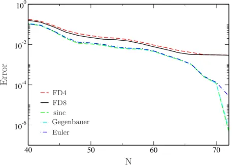
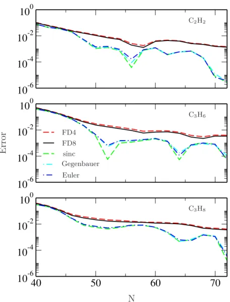
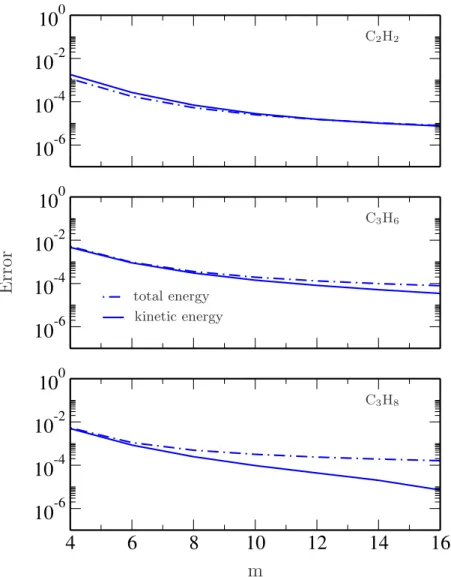
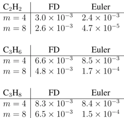
Computational Details and Results for Small Hydrocarbons
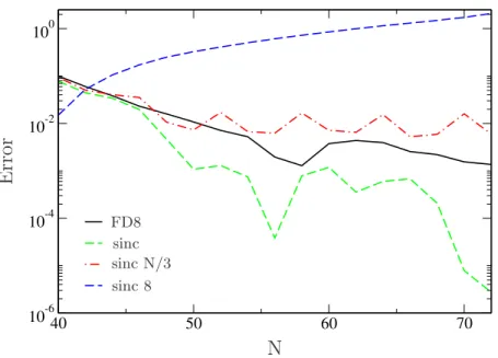
In this figure, the accuracy of the kinetic energy is compared with reference to that calculated using the full basis matrix N = 80sinc. The grid dependence for sinc calculations in this case comes from the local part of the pseudopotential.
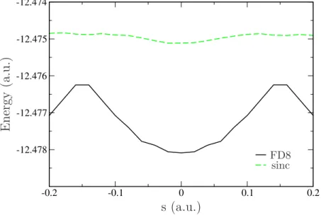
Summary
The eggbox effect is illustrated in the finite difference results, where the energy value fluctuates as the grid points shift. This construction effectively removes the dependence of the energy on the relative positions of the lattice points and ion centers.
Introduction
These techniques enable the separate evolution of the linear and nonlinear parts of the TDKS equation, allowing up to several orders of magnitude improvement in the accuracy of conventional techniques. Results of the exponential integrator methods applied to the description of different excitations of the one-dimensional helium atom and compared with those of the conventional time propagation techniques.
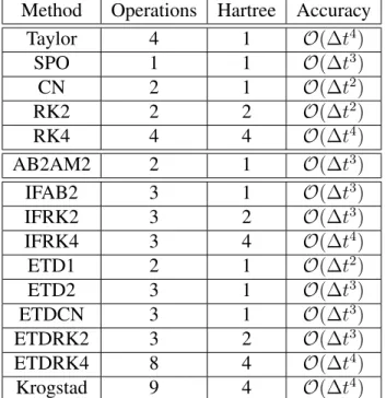
Propagation via Direct Numerical Integration
Here, the next step, ψ(tm+1) is approximated to the current step, ψ(tm), by taking a weighted average of the estimated slopes evaluated at the time steps between the two steps. This method shows a high computational cost, as four Kohn–Sham Hamiltonian estimates are required.
Propagation via the Time Evolution Operator
Taylor Expansion of the Time Evolution Operator
Such expansions are not unique to the Taylor expansion; another example is the Chebychev propagator [184, 185]. This truncation breaks the unitarity of the exponential, and the stability of the propagation becomes dependent on the time step size used.
Crank–Nicolson Approximation
The main advantage of this representation of the time evolution operator is that it remains unitary, so that the norm is explicitly preserved, barring rounding errors. Although iterative methods of matrix inverse computation allow for cases where entire matrices are stored, the application of the CN propagator is not feasible in real space grid approaches for large systems.
Split Operator Approach
This form is chosen so that each exponential of the matrix is diagonal in either real space or reciprocal space, facilitated by fast Fourier transforms. A final Fourier transform can then be used to return the representation to real space in which the final residual exponential is, again, diagonal.
Exponential Integrators
Integrating Factor Method
The purpose of this transformation is to improve the stiff linear part of the TDKS equations. The same scheme can be applied for the case of the second-order Runge–Kutta method (IFRK2) [205].
Exponential Time Differencing Method
By evaluating the inverse of the leftmost operator, one can arrive at another time propagation update scheme that approximates the discrete time step time evolution operator (ETDCN). It only differs from the above ETDRK4 method by the definition of the Ψ(a), Ψ(b), and Ψ(c) functions:.
Computational Details and Results for One-Dimensional Helium
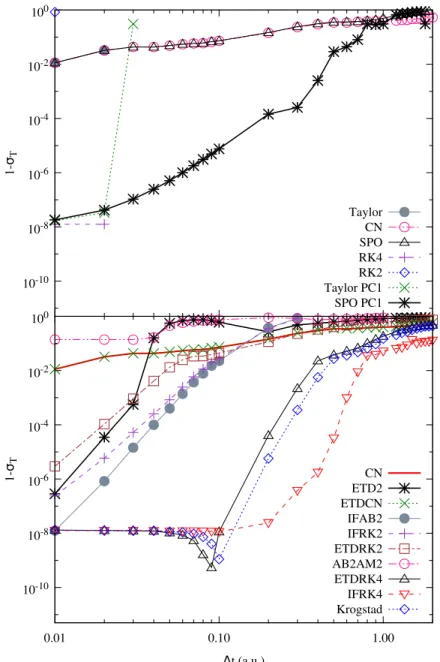
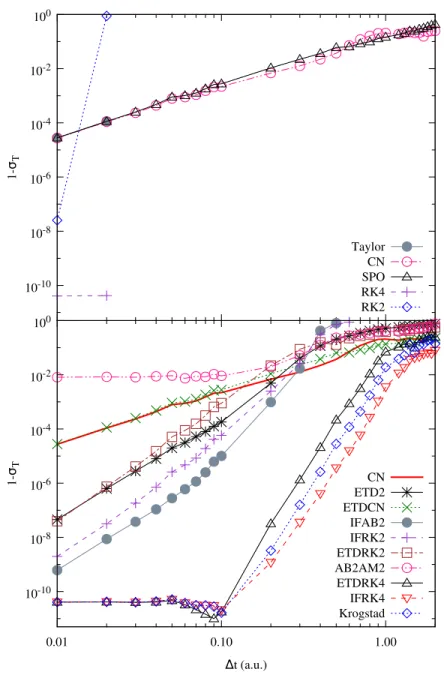
Excited State Superposition
As for the direct numerical integration methods, RK2 and RK4, they have fewer errors than the time evolution operator techniques, but are limited by a maximum time step size. The IF and ETD methods perform much better than the time evolution operator and direct numerical integration techniques, evidenced by smaller error for larger time step sizes.
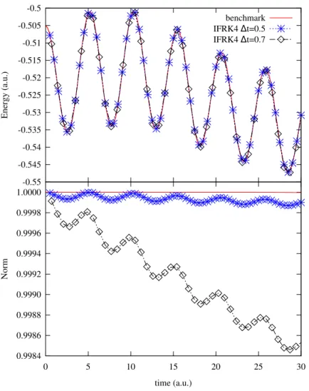
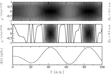
Laser-Driven Dynamics of a Single Orbital
Here, the time evolution operator and direct numerical integration methods fail to maintain accuracy over the course of the simulation. In the case of the time evolution operator and direct numerical integration methods, this increased error is due to large magnitudes of rapid change.

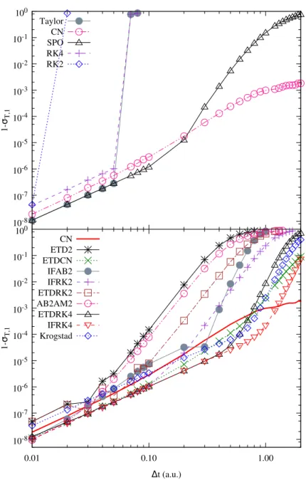
Laser with Two Orbitals
While the Taylor and CN approximations for the exponential time evolution operator degrade significantly in this case, the SPO approach performs best due to its analytical expression for the matrix-exponential form. While the SPO approach outperforms the out-of-time evolution operator methods, IFRK4 is able to match or outperform it for all choices of time step size, while other RK4-type methods maintain similar accuracy.
Summary
Of the IF and ETD methods, the IFRK4 and ETDRK4 approaches produced the most accurate results for each of the test cases. In cases where the dynamics were driven by the nonlinear part of the Hamiltonian, the RK4-type exponential integrator methods outperformed even the best-fit time-evolution operator methods by orders of magnitude.
Volkov State Basis Set
Without this mathematical displacement of the vector potential, this phase factor would still be present in the time dependence of the expansion coefficients of a static basis. The advantage of the Volkov mode expansion is therefore clear, as this phase factor can be analytically included in the definition of the basis functions rather than numerically propagated.
Computational Details and Results
One-Dimensional Mathieu Potential
6.4(c) and 6.4(d) for the same range of field strengths and frequencies and provide a more straightforward depiction of the Volkov state expansion's ability to better represent laser-induced dynamics. It can be concluded that the advantage of the Volkov state basis is best realized for field strengths above ~0.3a.u., which corresponds to.
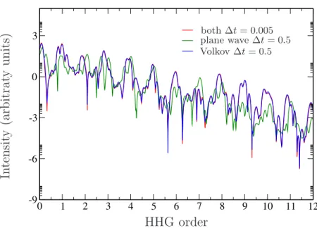
Three-Dimensional Bulk Diamond
Here, the increased magnitude of the current reduces the influence of fluctuations associated with the expansion of the Volkov base state. Even when using a time step size of 0.05 a.e. is the Volkov basis state propagation capable of distinguishing the modes associated with the third and fifth harmonics.
Application: Nano-Scale Vacuum Tube Diode
Model
The total length of the shape was then 20 ˚A, so as to give a volume corresponding to a cluster of 30 lithium atoms. The length of the box was adjusted to vary the separation distance between the peaks.
Results and Discussion
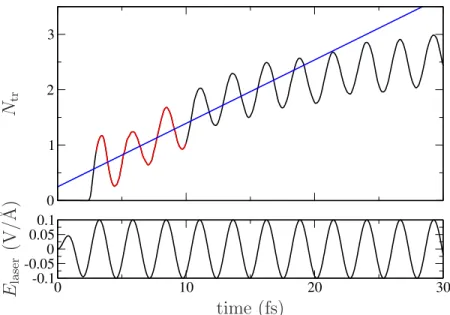
The resulting flux, determined at the location of the plane that bisects the two edges of the jellium model, z0. Here, positive values for Ntr relate to a transfer of probability density from sharp to flat edges of the jellium model, i.e.
Summary
An efficient implementation of time-dependent density-functional theory for the calculation of excitation energies for large molecules. Calculation of excitation energies within time-dependent density functional theory using auxiliary basis set expansions.