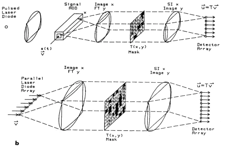
The many interesting discussions with the rest of the research group made the work with optical treatment at Caltech both stimulating and informative. Bits of the long signal are shot into the system with an acousto-optic device and spatially transformed across the device's aperture. Then, successively transformed parts of the long signal are multiplied by a reference and appropriately delayed and accumulated on a 2-D CCD to perform multichannel time integrations in the orthogonal dimension.
The one-dimensional linear transform of the desired high-time bandwidth is represented in the folded coordinate space of the 2-dimensional output detector. The operational characteristics of the main active devices used in these time-space integrative systems are examined from the perspective of the system architect. The effects of devices on overall system operation are discussed and device designs intended for application in a time- and space-integrated system operating environment are proposed.
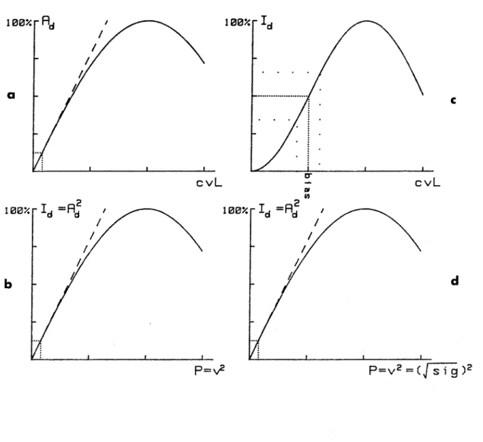
These include spatial carrier coding of the interferometric terms combined with bandpass filtering, and direct bias subtraction techniques. Linearity of the high spatial bandwidth chirp transform processor Phase-averaged impulse response of the TDI chirp transform processor.
INTRODUCTION
This vision has become practical due to the simultaneous maturation of three technologies; optical laser diode sources, acousto-optic (AO) traveling wave modulators and two-dimensional charge-coupled device (CCD) detector arrays. An essential feature of the processors considered here is that signals flow dynamically through the processor, and it is both the spatial and temporal variations of the optical modulations that are used to perform the two-dimensional processing operations. In Chapter 2 I begin with an overview of the simple model for the operation of an acousto-optic (AO) Bragg cell as an optical traveling wave modulator.
One-dimensional time-delay integration (TDI) correlators are discussed, which take advantage of the drift capability of optical detectors of charge-coupled devices. The general performance limitations of the hybrid time-space integration technique are shown. Laser diodes (LDs) are used as the optical source in the experiments presented in this paper due to the ease with which they can be directly modulated at high speeds or pulsed with narrow pulses.
One-dimensional systems are simply not large enough to contain all the signal information that must be Fourier transformed by the spectrum analyzer, so the signals are fed into the system a small portion at a time. A simpler system using a TDI CCD detector array to perform time-integrating chirp transforms on each resolvable channel of the space-integrating spectrum analyzer was also tested.
ACOUSTO-OPTIC SIGNAL PROCESSING
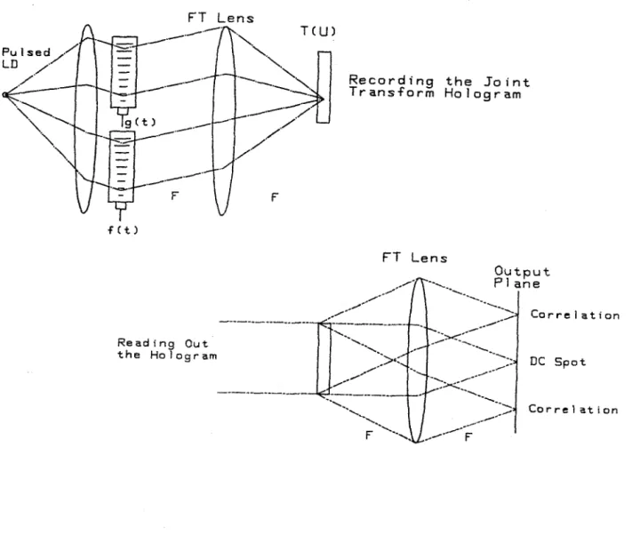
Often we will use this window function in a coordinate system with reference to the center of the AOD where x' = x - X/2. The last term is the Fourier domain representation of the matched filter for the image g(x-xo,y-yo). It states that the product of the Fourier transform of two signals is equal to the Fourier transform of their convolution.
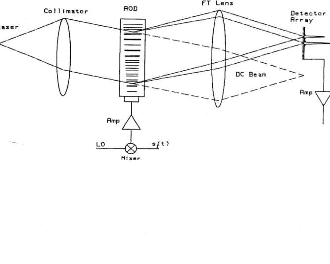
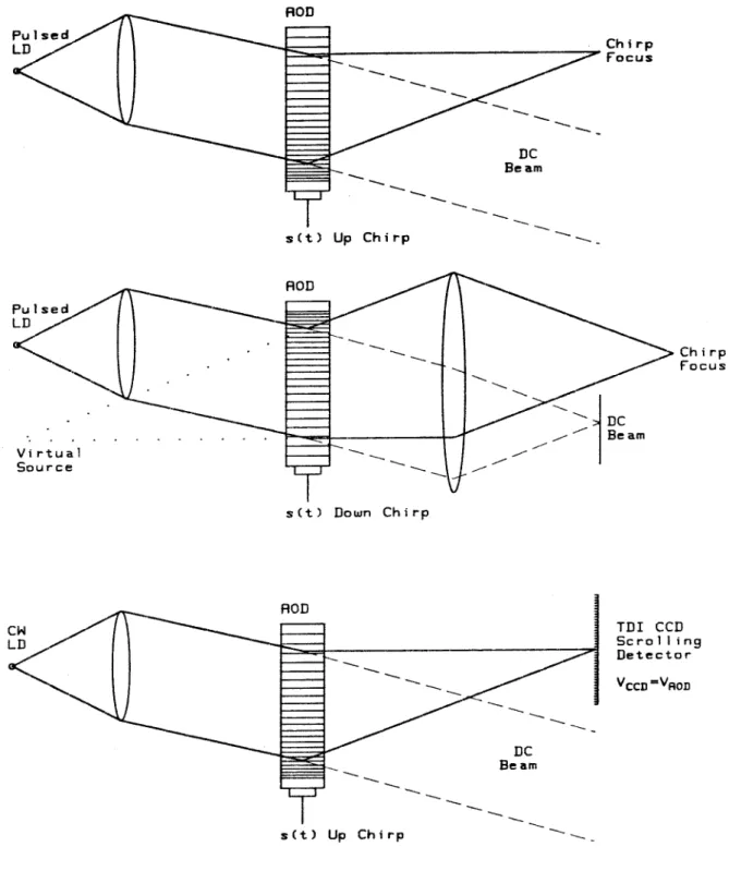
The signal applied to the AOD transducer is s(t) and the diffracted signal is given by the product of the incident illumination with the traveling wave single sideband amplitude modulation of the AOD. This results in the condition that the laser pulse width r < 2/B, where Bis the bandwidth of the AOD. The second term is centered at the position x' = k:i>.F, and is a spatial representation of.
Placing a small high bandwidth output detector in the focal plane will produce a time domain output of the chirp correlation. For the autocorrelation of two signals with two-sided bandwidth B, the condition Jo > applies. The signal accumulated on the detector array after N laser diode pulses is given by the time integration of the product of the source modulation with the diffracted intensity of the AOD.
The final identity leads to the symmetric counterpropagating implementation of the chirp algorithm, and does not require a chirp postmultiplication.

TIME AND SPACE INTEGRATING SIGNAL PROCESSING
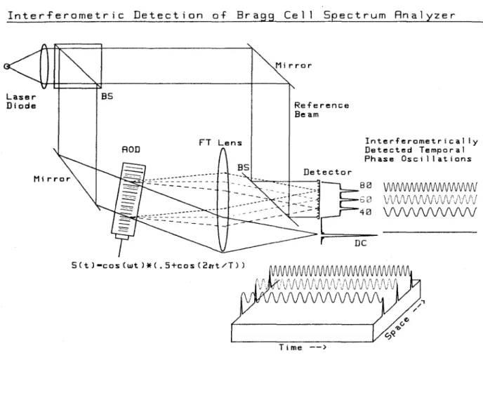
Various subspace projections of the time-frequency representations can be performed with multidimensional integrations, such as time-averaged in-. The multiplication between the signal and reference wavefronts is accomplished as a cross term in the interferometric detection of the recombined wavefronts. The last term is the desired heartbeat between the signal and the complex conjugate of the reference.
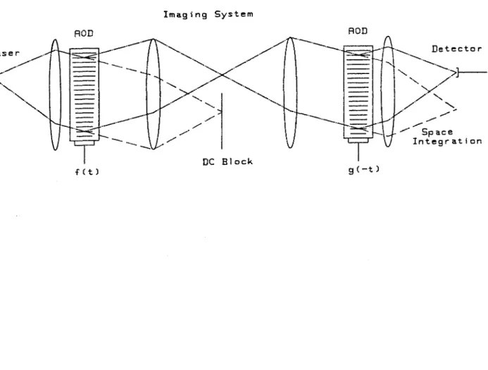
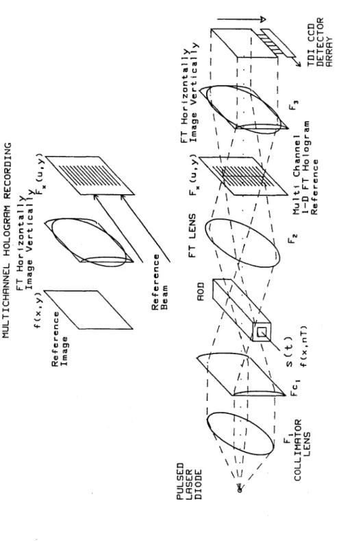
The system effectively calculated the correlation (or convolution) of the input signal with the image stored in the multichannel reference hologram in real time. Demodulation of the interferometric term on the spatial carrier will produce the desired image Fourier transform. In this equation, we can associate a specific element of the input matrix F(m0 , no), (or pixel of the input image) with a space-variant impulse response matrix (or image) of the transformation tensor H(mo, no, i,j).
In this equation we can associate a certain element of the input vector !(lo) with the corresponding row in the transformation matrix H (k, lo). The corresponding continuous representation of the linear system of the space variant is given by an integral transformation. In this expression, Rn(!) is the temporal Fourier transform of the information of duration 2T in the nth raster line, while R(f) is the Fourier transform of the.
All other diffracted terms from the multichannel hologram contribute to the normal sidelobes associated with the r(t) waveform. A classic example of such a transform kernel is the Fourier transform, and this type of decomposability of the Fourier kernel results in When the ordinate of the output frequency is represented as a basis equal to the square root of the total resolution.
This description sounds identical to how a Fourier transform image system works, but there are critical differences. It also represents an almost ideal match with the capabilities of the TSI processing technique. The approach used in the TSI processor is based on the sequential processing of the distance and azimuth dimensions.
In this approach, the focal length range of the film is constant, FR = Vk/b>.0. The dimension chosen to represent the carrier frequency will suffer a reduction in the available resolution capabilities of the detector array.
DEVICE PERFORMANCE FOR TSI SIGNAL PROCESSING
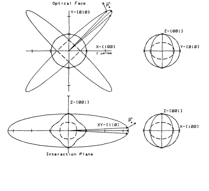
Acoustic eigenmodes
The acoustic wave is modeled as a time and space varying particle displacement vector field it( x, t), which at each crystal lattice location describes the particle displacement from its equilibrium position!9,ioJ. A sinusoidal displacement wave of amplitude W, radial frequency n, wave vector IKI A, acoustic wavelength A, propagating with a phase velocity va(S) = O/IKI in the direction defined by the unit vector s = K / IKI, and with unit polarization . The symmetric part of the displacement gradient matrix is known as the linearized Strain tensor and its components are given by
The stress tensor Tij', which is symmetric in non-feroic materials, is related to the stress tensor via the elastic stiffness tensor of the 4th rank in a generalization of Hooke's law. 4.2.4) Where the Einstein summation convention for repeated indices is implied, and i, j, k, l can take any of the three spatial directions x1, x2, x3 or equivalently x, y, z. The elastic coefficients have certain symmetries due to the symmetry of S and T, so that Cifkl = Cfikl = Ciflk = Cfilk, and energy arguments show this.
The acoustic field equations show that energy oscillates between the. strain energy and strain energy in a manner analogous to the electromagnetic oscillation between electric and magnetic energy. The dynamic equation of motion for a vibrating medium relates the restoring force as given by the divergence of the stress tensor to the mass times acceleration of the displacement field. Substituting the stress-strain relationship and the definition of stress in terms of particle displacements into the dynamic equation of motion results in the differential equation governing the propagation of particle displacement fields.
This system is compatible for all waves only if the system determinant is zero, which results in the dispersion relation in terms of the Christoffel matrix fik(S) = CijklSjSl as a function of the direction of propagation 8, where S:r, Sy, Sz are the proper direction cosines. sea lri;iS) -PmOikl. This equation has three solutions for the acoustic slowness, or inverse velocity 1/va(S) = K/0 for each direction 8, forming three scaled surfaces of equivalent frequency in K space, known as acoustic momentum space.