For example, the term map, historically a punch map, must be interpreted as a line of the input file. For this reason, this tutorial document has been prepared to introduce the beginner to the more basic (and essential) aspects of the MCNP code.
Annotating the Input File
The MCNP documentation is very extensive; Thus, it is difficult for new users of the Code to distinguish between information that is essential to learning to use the Code and information that is only needed in very specialized circumstances. A continuation line starts with 5 empty columns or a blank followed by an & at the end of the card to be continued.
Units Used by MCNP
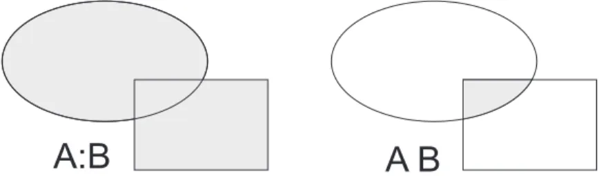
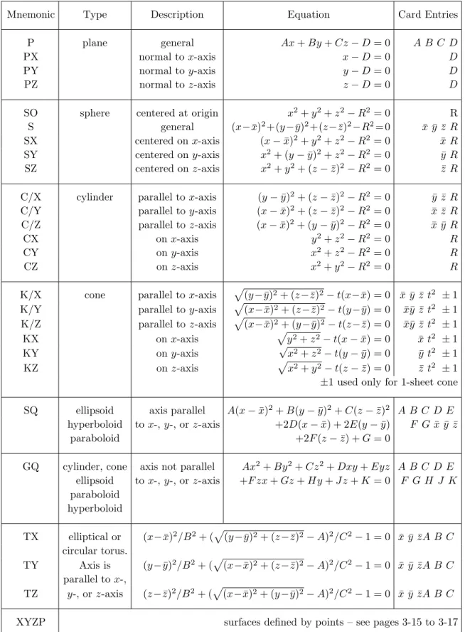
These directional senses for the surface are formally defined as follows: any point at which f(x, y, z) > 0 is located in the positive (+) sense of the surface, and any point at which f(x, y, z )<0 is found in the negative sense (−) with respect to the surface. For example, the area inside a cylindrical surface is negative with respect to area and the area outside a cylindrical surface is positive with respect to area.
Cells – Block 1
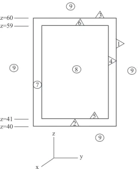
This volume is negative with respect to surface 4, positive with respect to plane 5, and negative with respect to plane 6. This "graveyard" cell, say cell 9, is the union of all positive regions with respect to surfaces 1 and 3. and negative with respect to surface 2.
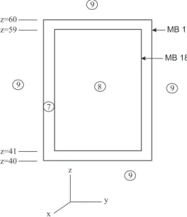
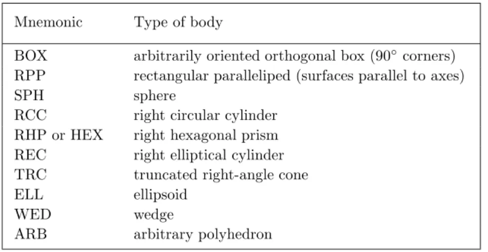
Macrobodies
Specification of materials that fill the various cells in an MCNP calculation includes the following 3-114 to 3-124 elements: (a) defining a unique material number, (b) the elemental (or isotopic) composition, and . c) the cross-section compilations to be used. Here, 1001 and 8016 provide atomic number and atomic mass designations, in the form of the ZAID numbers.
Cross-Section Specification
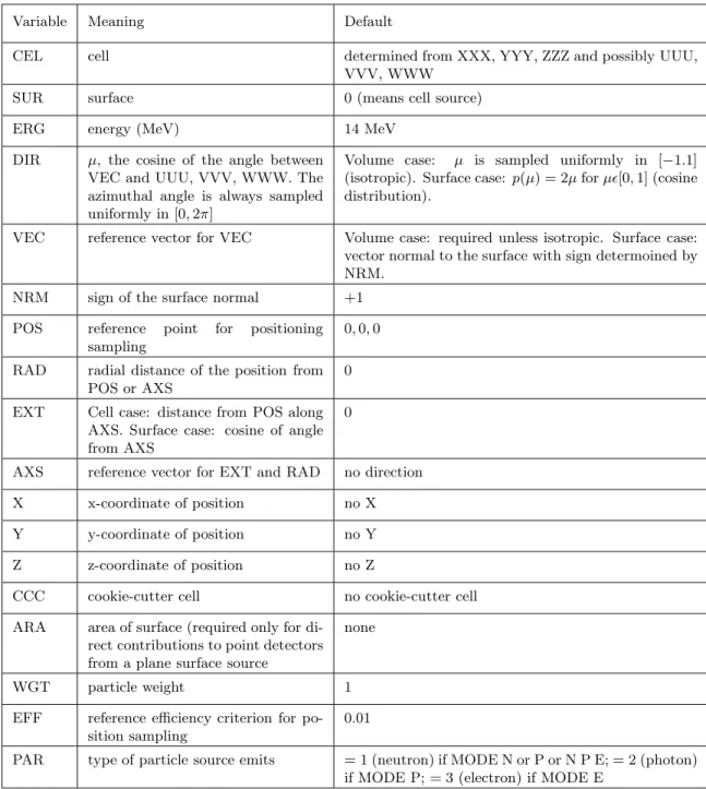
Source Specifications
- Point Isotropic Sources
- Isotropic Volumetric Sources
- Line and Area Sources (Degenerate Volumetric Sources)
- Monodirectional and Collimated Sources
- Multiple Volumetric Sources
Points, randomly chosen c on the rectangular parallelepiped, are accepted as source points c only if they are inside cell 8. c. Points, randomly selected on the sphere, c are accepted as source points only if they are inside cell 8. To normalize the number per source particle to the cone, set WGT=1/fsa2 in the SDEF card, where fsa2 is the fraction of the solid angle. of the cone (0.05 in the example above).
The rejection technique is used to select the source points c with cells 8 and 9 with the specified frequency. A random point inside a cylinder c is accepted as a source point only if it is inside the source cell c. The location and size of the sampling cylinders and the source photon energies c are functions of the source cell (FCEL).
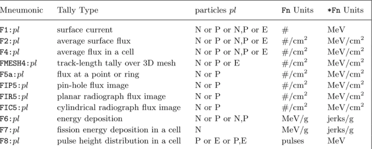
Tally Specifications
- The Surface Current Tally (type F1)
- The Average Surface Flux Tally (type F2)
- The Average Cell Flux Tally (type F4)
- Flux Tally at a Point or Ring (type F5)
- Tally Specification Cards
- Cards for Surface and Cell Tallies
- Cards for Point-Detector Tallies
- Cards for Optional Tally Features
- Miscellaneous Data Specifications
- Short Cuts for Data Entry
Technically, if Φ(r, E,Ω) were the energy and angular distribution of the fluence as a function of position, the F2 counts would measure. Technically, if Φ(r, E,Ω) were the energy and angular distribution of the fluence as a function of position, the F4 counts would measure. The values of X, Y, and Z indicate the coordinates of the point detector, and R indicates the radius of a spherical exclusion zone surrounding the detector point.
The manual also describes the use of a ring detector – useful for problems with symmetry around one of the problem axes. A table on page 3-77 of the MCNP manual lists many optional commands that change what corresponds to Sec. The Energy Multiplier Card Optionally associated with the tally energy card is an energy multiplier 3-98 (EMn) card of the form.
Running MCNP
Execution Options
Mode Card This card is used to specify the type of problem, i.e., the type of source particles in 3-24. When mode is specified, the PAR entry can be omitted in the SDEF resource definition card. Time or History Cards The usual method to limit the runtime of MCNP is to specify either 3-133 .
In addition, or as an option, the calculation time cutoff, in minutes, can be specified by card 3-134. The Print-and-Dump Cycle Map By default, an output file is created only at the end of a 3-136. With this card, a maximum of 60 minutes of computer time will be lost if a calculation is cancelled.
Interrupting a Run
In the first approach, the model geometry and physics used to simulate particle transport can often be simplified or shortened. For such a problem, once a neutron leaves the fast energy region, it can be killed without affecting the calculation. The second basic approach to reduce the variance of a calculation is to modify the simulation process itself by making certain events more or less likely than they actually occur in nature.
These non-analogous tricks can be categorized into three general methods: (1) population control, (2) modified sampling, and (3) partially-deterministic calculations. In population control, for example, the number of particles in regions of high/low importance can be artificially increased/decreased. Finally, in the partially-deterministic methods, part of the random walk simulation can be replaced by a deterministic point-kernel type calculation.
Tally Variance
Relative Error and FOM
In any variance reduction method, we change the simulation and therefore change the underlying 2-109 to. By making p(x) more concentrated around its mean (which remains the same as the mean of the analog PDF), the variance of the mean of Sx2 will be smaller than that of the analog PDF, i.e. our estimate of the mean will be more accurate. As described in the manual, R generally needs to be less than 0.1 to get meaningful results (and even less if point/ring detectors are used).
This property of the relative error is the major weakness of the Monte Carlo method, because generally many histories must be generated to obtain acceptable results. Since R2 ∼ 1/N we see that the FOM should remain relatively constant except at the beginning of the simulation. Also, for different simulations of the same problem, the simulation with the largest FOM is preferred because it requires the least time or produces a specified relative error.
Truncation Techniques
Energy, Time and Weight Cutoff
The CUT command is used to determine the minimum energy, time, or particle weight below which a particle is 3-131 killed. The first is the per-history time limit, which in the example above is specified as jto skip the default value of very large time. ELPT is like the CUT card, but allows you to set a threshold value for each cell individually.
If the ELPT and global CUT commands are used, the higher limit prevails. The CUT and ELPT commands are particularly useful for energy deposition calculations to which low-energy particles make little contribution. However, for neutron problems, use CUT and ELPT with caution since low energy neutrons cause most fissions and produce most gamma capture photons.
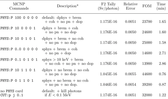
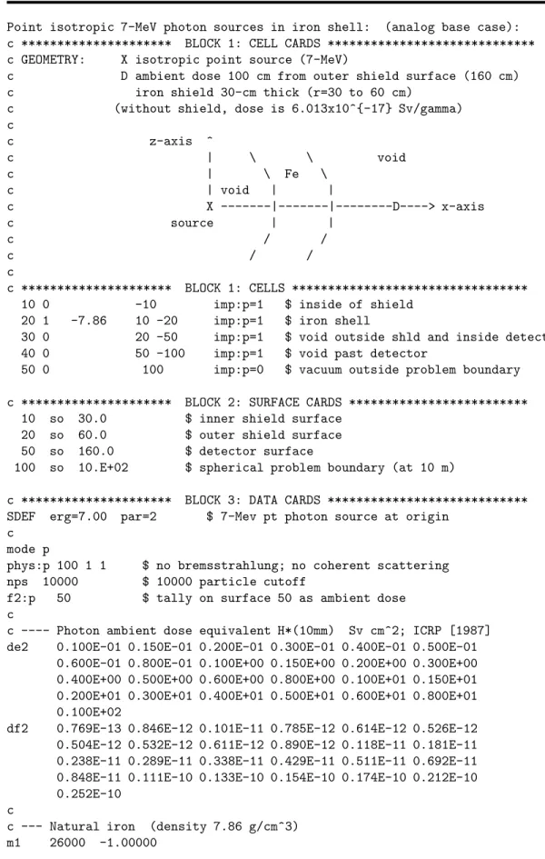
Physics Simplification
Neutrons: MCNP with its integrated neutron cross-section libraries is an ideal tool for neutron transport research. For neutrons, the PHYS card has only four parameters, namely PHYS:N EMAX EMCNF IUNR DNB. The EMAX parameter is the energy in MeV above which neutron data is not placed in memory (default is very large).
If IUNR= 1, cross sections averaged over the region of the resolved cross section are used, while if IUNR= 0 (the default), probability tables are sampled that describe interactions in the myriad levels and widths of unresolved resonances. PHYS:n 5.0 0.1 $ maximum sigma table energy; analog capture below 100 keV Only cross section data below 5 MeV are retained here (to save data storage memory). For neutrons below 0.1 MeV, analog absorption (direct simulation) will be used, and above 0.1 MeV, implicit absorption.
Histories and Time Cutoffs
Nonanalog Simulation
Simple Examples
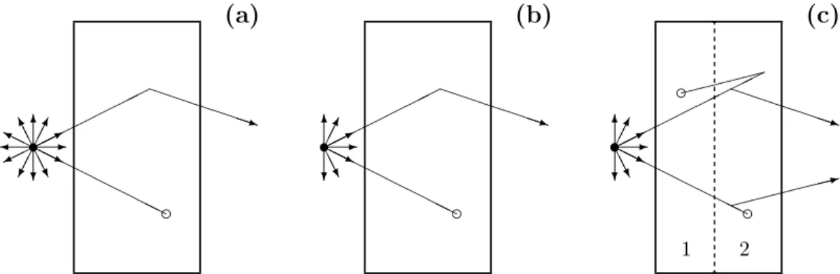
For the same number of source particles, twice as many reach the tally surface in case (b) compared to case (a), and thus the variance of the case (b) tally is smaller. When a particle crosses from the layer closest to the source to the layer closest to the number surface, it splits into two particles, each with half the weight of the original particle and both moving at the same speed as the original particle. Twice as many particles will now reach the counting surface (thereby reducing the variance of the count); but since their weights have been halved, the expected numerical value remains unchanged.
Russian Roulette: When a particle reaches a region of space far from the counting range, it is unlikely, with additional random walk simulation, to reach the counting range, and the running time can be reduced by terminating or killing such a particle. In the example case (c), when a particle in the right substrate returns to the first left substrate, we might think that it has a relatively poor chance of returning once more to the right substrate and reaching the thallic surface. Implicit Absorption: The particles that are tracked through the slab but absorbed before reaching the overview surface represent wasted computing effort.
MCNP Variance Reduction Techniques
- Geometry Splitting
- Weight Windows
- An Example
- Exponential Transform
- Energy Splitting/Russian Roulette
- Forced Collisions
- Source Biasing
In the following sections, some of the simpler variance reduction techniques are discussed and illustrated. Of course, in any division or Russian roulette, the weight of the remaining particles is adjusted to leave the calculation unbiased. To use the weight window generator, the commands WWG (and, optionally, WWGE) are placed in block 3 of the input file.
Near the end of the output (and in filewwout), produce the weight window cards shown in the middle of page 29. Then place the generated weight window cards written near the end of the output in Block 3 and reopen the problem using a simulation biased weight window. When such a particle is created, the ESPLT command can be used to split the particle into more daughter particles of the same type.
Final Recommendations
Herefi is the fraction of the solid angle for the ith cone and is calculated asfi= [µi−µi−1]/2. 72(b) Cell Temperatures 170 Source Frequency; surface source 85 Electron range & straggling 175 Estimatedkef f by cycle 90 KCODE source data 178 Estimatedkef f by batch size 98 Physics const. & compilation options 180 WWG accounting summary.
Accuracy versus Precision
Tally type: The choice of tally type often greatly affects the precision of the results. Variance reduction: The use of various variance reduction techniques can greatly affect counting precision. Number of stories: The more stories run (and the greater computing effort used), the better the precision of the counts.
Statistics Produced by MCNP
- Relative Error
- Figure of Merit
- Variance of the Variance
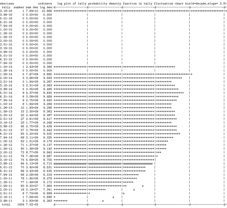
- The Empirical PDF for the Tally
- Confidence Intervals
- A Conservative Tally Estimate
- The Ten Statistical Tests
- Another Example Problem
The estimate of the relative error R is important to indicate the accuracy of the average. The VOV includes the third and fourth moments of the distribution f(x) and is much more sensitive to fluctuations in large historical scores than isR, which is based only on the first and second moments off(x). MCNP also constructs the tally PDF f(x) to help assess the quality of the confidence interval estimates for the tally mean.
It is for this case that MCNP performs an extensive analysis of the high tail of the PDF counts. MCNP uses the histories of the highest scores (the 200 largest) to estimate the slope of the high tail of the PDF. The mean should show, for the last half of the problem, only random fluctuations as N increases.