Introduction
General remarks
This thesis addresses three different problems at the intersection of analytic number theory with adjacent areas, including harmonic analysis, automorphic forms, spectral theory, and dynamical systems. This conjecture, which combines multiplicative number theory and dynamical systems, has seen spectacular progress in recent years.
Context and description of results
It is tautological that the expected value is equal to the RHS of the same equation. The key point is that the term ∆f(s) +bχ0,a·∆f(s, χ0) has the same poles as ∆f(s) inside the critical band.
Simple zeros of GL(2) L -functions
Introduction
An adaptation of that method for degree n = 2 also implies that a positive part of the zeros lies on the critical line [2], but already cannot handle simple zeros and only shows that a positive part of the zeros of the order of a maximum of three. [34]. It roughly consists of the possibility that Λf(s) has simple zeros arbitrarily close to the line <(s) = 1.
The setup
To rule out pole cancellations in (2.4) for any α ∈Q×, we introduce a new number-theoretic input to the argument, namely a zero-density estimate for f-curves. Taking the inverse Mellin transform of ∆f,a,q (evaluated at −iz), shifting the integration line to the left of the critical bar - where we get the factor Sf,a,q corresponding to the poles - and giving using the functional equation (Proposition 1) to return to the right of the critical bar, we obtain (see [12, Lemma 2.3] for details) the relation.
Existence of poles of H f,α
This indeed follows from (2.12) and the fact that for non-trivial χ (mod q) the poles of. As a consequence, we can also understand the poles of ∆f,a,q(s) with<(s)≤0, through the functional equation.
Location of poles of H f,α
A standard argument using Perron's formula then gives the desired contradiction, so we conclude that Gf,p(s) has at least one pole in <(s)∈(0,1), as desired. We will show that there exists a prime number p that satisfies p ≡ 1 (mod N), so that ρ is a pool of Hf,1 or Hf,1.
An improved estimate for f of level 1
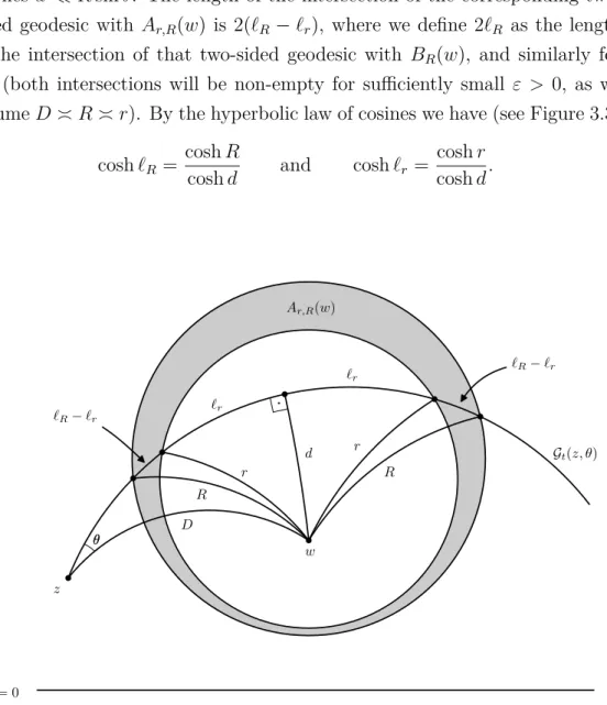
This is the same issue that creates a continuous spectrum in the spectral solution of the inX Laplacian. The length of the intersection of the corresponding two-sided geodesic with Ar,R(w) is 2(`R−`r), where we define 2`R as the length of the intersection of that two-sided geodesic with BR( w), and similarly for 2`r (both intersections will be non-empty for sufficiently small ε > 0, as we assume DRr). The proof of Theorem 4 actually yields an energy-conserving error term of the form Oε(D12R3+ε) for any sufficiently small ε >0 (depending on δ).
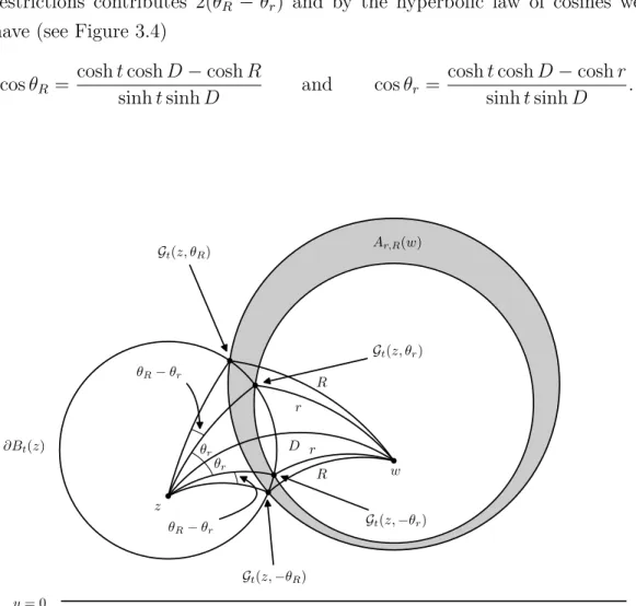
If one has an upper bound of the (expected) correct order of magnitude for the variance, i.e. Note that the integrand in (4.4) is independent of the second coordinate, so we can rewrite the integral as More than two fifths of the zeros of the Riemann zeta function are on the critical line.J.
The variance of closed geodesics in balls and annuli on the
Introduction
Such an expression was first studied by Bourgain, Rudnick and Sarnak [16] in the context of grid points in spheres. Furthermore, in the case of closed geodesics, they obtained the same distribution for almost all rings by showing that if0≤r < R1. However, in retrospect, such a result is quite reasonable, since geometric invariants have codimension 1 in the case of closed geodesies, and 2 in the other mentioned cases.
The main result in this direction is Theorem 3, where, in the case of spheres, we show that for a single random geodesic segment of length LinΓ\H under mild conditions, the appropriate expression for the variance is ~ 16LRπ 3. For rings, a special function is determined and appears in the asymptotics (see lemma 13 for its definition and key properties). Especially in the case of balls, we assume that if 0< R≤D−δ for some fixed δ >0, then.
Background and notation
LetX := Γ\Hdenote the modular surface, so that our previous identification quotients go out to X ' Γ\G/K, and similarly for the unit tangent bundle1 identification T1(X) ' Γ\G. Both measures are G-invariant under multiplication on the right, as the specific choice of fundamental domain turns out to be unimportant. To interpret the unit tangent bundle T1(X) correctly, we need to consider the orbifold structure of X, but this minor problem can be safely ignored for our purposes.
Once again, Get preserves eν and corresponds to parallel transport of (hyperbolic) signed length t along the corresponding geodesic in X .
Estimates for the Selberg–Harish-Chandra transform
We restrict our attention to the caseR−r R, which will be relevant to us, but a similar statement also holds in the complementary case. The reason we keep an expression with Bessel functions in the result above, instead of using (3.4) as in [54, Lemma 2.27] to write it in terms of simpler trigonometric functions, is that the main term in our variance calculation will come roughly from |t| 1/R. The main difference between the two cases is the presence of the additional weight H(t) given by (3.22) in the spectral expansion of the variance for closed geodesics, which is not present in the case of Heegner points considered by Humphries and Radziwiłł ( see [54, Lemma 2.13] for a comparison of the two weight functions).
Variance for random geodesic segments
The tube SR has few self-intersections in that case, and the geometry of the problem is essentially Euclidean (as we. Therefore, our situation can be modeled by the toy problem where the geodesic segment S is replaced by a straight line segment of length L in R2 , and the point w is random over some region of the appropriate area µ(X) = π3 containing the (now Euclidean) tube SR. In view of the necessity to exclude the contribution of the point, we let FA :={z ∈ F :=(z)≤A}.
Therefore we can assume that r≥ R2, and then a slight modification of the argument above also takes care of D≤ R4, since sinht sinhR in that case. Indeed, the integrand for each θ is now the length of the intersection of the one-sided geodesic determined by (z, θ) with. Note that since π(g) ∈ Ar,R(γ0w) we can restrict the integral over t to [−2R,2R], since the intersection of a geodesic with an annulus Ar,R in H in a segment of the geodesics of length ≤ 2R.
Variance for closed geodesics
The restriction R−r R in Theorem 4 is mostly technical due to the fact that the behavior of the weighting function hr,R(t) changes when R−r R. The error is estimated using the bounds and asymptotics in Lemma and Lemma 22, while considering each of the scopes separately. Then (3.29) allows us to complete the integral up to (0,∞) under the same error term as above.
To conclude the proof of Theorem 4, it suffices to show that the shifted convolution (3.38) is asymptotically smaller than the leading term obtained in the previous subsection. This requires considerably more work and involves a more precise treatment of the fluctuation of the test function h(t). We will divide the integral in (3.43) into three different regions for x and bind each separately.
Limitations and connections to subconvexity
As a side note, we note that here the meaning of the exponent 5/12 in Theorem 4 becomes clear. An improvement in the first-moment bound (3.53) essentially corresponds to an extension of the range of R in Theorem 4. In fact, we prove in Section 4.5 that if one only assumes that φ ∈ C1 then, at least along the sequence of best rational approximations of the irrationalα, the stiffness rate ofTα,φ can be logarithmic even whenφ(0) = 0b.
The proof is a simple modification of the proof of Lemma 26, replacing qεn by ψ(qn), so that for example `n∈Z is chosen such that. It is noted that we do not have multiplicity of ψ, therefore the relation is not of the form ψ(rn)−1/100, but it suffices to prove that Tα,φ is rigid3 (the last limit can be obtained if we set additional conditions for ψ ). If f ∈ C1+ε, then all special flow maps Tf ={Ttf}t∈R onto the irrational rotation Rα are Möbius disconnected.
Möbius disjointness for C 1+ε skew products
Introduction
A common feature of all the listed results is that the underlying system is regular, in the sense that for every x∈X the sequence N1 P. Difficulties in dealing with every such ν are overcome because they all project onto the Lebesgue measure in I coordinate the first one. In Section 4.6 we show that our ideas can be used to extend some general stiffness results so far known only for zero-mean functions in the general case.
Finally, in Section 4.7 we use our argument to derive new Möbius incoherent results for flows in T2 and Rokhlin extensions. We also abbreviate e(x) :=e2πix and use the asymptotic notation f(x) g(x) (respectively f(x) p g(x)) to mean that there absolutely exists C > 0 (respectively just depends from the parameter p) such that |f(x)| ≤ C|g(x)| for all x in the relevant range. I am also grateful to the American Institute of Mathematics (AIM) for their 2018 workshop on "Sarnak's conjecture".
Reduction of disjointness to a rigidity result
Continued fractions and some arithmetic estimates
Using the Denjoy-Koksma inequality for sums over r as in the proof of Lemma 27, since R .
Polynomial rate of rigidity in C 1+ε
In our choice of {en}n1 contributes high in the first term in the RHS of (4.4).
Counterexample to polynomial rate of rigidity in C 1
Taking the terms corresponding to tok = n and k = n + 1 in (4.12), respectively, and using the positivity of the other terms, we conclude that the whole expression is (logqn)−4, so there is no polynomial convergence rate to zero along a subsequence of {qn}n≥1. In fact, [64, Lemma 3.2] shows that a decay of the form exp(−(log logqn)1+δ) for any δ > 0 would suffice for Möbius incoherence, but that too is false according to our counterexample.
Extension of general rigidity results to φ of non-zero mean
If α ∈ R\Q and φ are absolutely continuous of topological degree zero, then the tilted product Tα,φ is uniformly rigid. We can simply use the original result for the zero mean case to conclude that there exists λ(n)→ ∞ asn → ∞ such that. With the above conditions, we can show that there exists a sequence of positive integers {rn}n≥1 such that.
If φ : T → R is of class C1+ε, then there exists an unbounded sequence of positive integers{rn}n≥1 such that. You can show it with the same techniques as in the corresponding results of section 4.3, but this time for the functions. For example, an approximation of Proposition 9 using L∞ methods would already be frustrated by the presence of the extra logarithmic factor in (4.13), if the decay of the Fourier coefficients is slow enough.
Smooth flows on T 2 and Rokhlin extensions
The purpose of this appendix is to obtain a zero-density estimate for character twists of a fixed formf that holds in the generality required for our application in Chapter 2 and is efficient in the Q-aspect. Proposition 11 is not particularly efficient in the T aspect, but this is irrelevant since T is fixed in our desired application. We want it to be Oε(L−2), which holds if, for example, it is assumed. A.18) To unify the treatment of the sum and integral, we consider the measure.
From now on, the only properties of the coefficients we will use are that they do not depend on s or χ and satisfy af(n, v)d4(n). Optimal small-scale even distribution of grid points on the sphere, Heegner points and closed geodesics. Jutila. Lectures on a Method in the Theory of Exponential Sums, Volume 80 of the Tata Institute of Fundamental Research Lectures on Mathematics and Physics.
Closed geodesics in Λ D
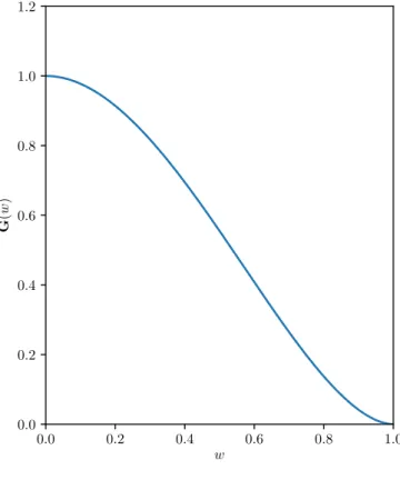
Graph of G(w)
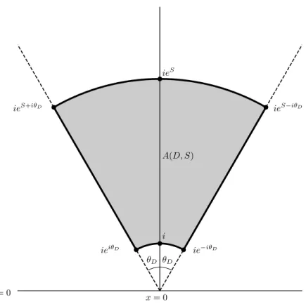
The region A(D, S)