This leads us to the effective Lagrangian chiral perturbation theory for low-energy interactions of light pseudo-scalars. Another important global symmetry is the SU(NJ)L x SU(NJ)R chiral symmetry of the QCD Lagrangian tree level with NJ massless quark flavor. This symmetry leaves such a Lagrangian invariant under particular global transformations SU(NJ)£ and SU(NJ)R of the left- and right-handed quark fields, respectively.
For example, breaking the local SU(2) x U(l) electroweak symmetry via the Higgs mechanism has provided the Standard Model with a possible, although still experimentally unconfirmed, explanation for the behavior of the weak and electromagnetic interactions in a uniform context [ 4]. Breaking the chiral symmetry SU(NJ)xSU(NJ)R of the QCD Lagrangian is an important example of global symmetry breaking, and has several applications in studying the strong interactions of low-energy hadrons.
Chapter 2 Chiral Symmetry: Concepts and Formalism
Spontaneous Global Symmetry Breaking and Goldstone Bosons
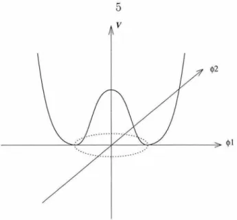
It is instructive to parameterize the field
We observe that, based on a theory that has a U(l) symmetry, by spontaneous symmetry breaking, we have ended up with a massless e-particle. This is a general phenomenon, that is, the spontaneous breaking of a continuous global symmetry results in the generation of one or more massless scalar fields.
Chiral Symmetry in QCD
These experimental facts suggest that the vacuum of the theory does not have the symmetries of the classical Lagrangian and that chiral SU(3)L x SU(3)R is spontaneously broken. As mentioned before, the smallness of ( u, d, s) quark masses suggests that the explicit symmetry breaking due to mass terms of the form m(ff.LqR + fi.RqL) is not severe in ( u, d, s) sector. These are the eight lightest pseudo-scalar mesons, corresponding to the eight broken generators after spontaneous chiral symmetry breaking; SU(3)L x SU(3)R ---+ SU(3)v.
Since the ground state of the theory in strong interactions is not invariant under the SU(3)L x SU(3)n chiral group, we have. where QA = QR, - Q'l are the axial load operators, and Ob if.15>.bq are the operators representing light pseudoscalars. In the next section, we will show how the Goldstone pseudo-boson interactions can be formulated in terms of an effective Lagrangian that incorporates the features of the QCD Lagrangian that were discussed above.
Chiral Perturbation Theory
Since we are interested in the low-energy regime of hadronic interactions, we construct an effective chiral Lagrangian for light pseudoscalars from a minimal number of derivatives. In the chiral limit, where quark masses are zero, pseudo-Goldstone bosons, which are mesons, are massless. Higher-order terms can be systematically added to the Lagrangian in the derivative expansion.
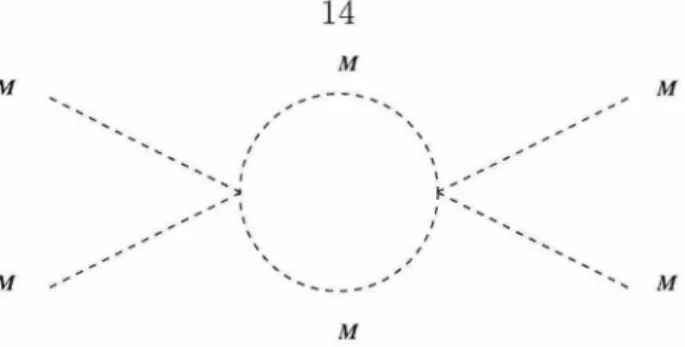
For example, using the O(p2) vertex operators, a 1-loop computation requires the inclusion of tree-level O(p4) terms that act as counterterms in the renormalization of the loop diagrams. The loop integral can be controlled in the ultraviolet by a cutoff AxB, the scale above which the effective chiral Lagrangian becomes unreliable.
Chapter 3 Chiral Perturbation Theory
- Chiral Perturbation Theory for Vector Mesons
- Differential Decay Rates
- Summary and Remarks
- Chapter 4
This chapter aims to illustrate the utility of heavy vector meson chiral perturbation theory for T-decay. In the next section, we derive the hadron level operators that represent these currents in chiral perturbation theory. In the chiral perturbation theory of heavy vector mesons, their widths appear as antihermitian terms in the Lagrangian density (3.9).
15], the widths could be neglected in the propagator at leading order in chiral perturbation theory. Our expression for the invariant matrix element in Eq. 3.24) is derived using heavy vector meson chiral perturbation theory, which is an expansion in m1f/mp and v · p1f/mp. It seems reasonable that the lowest order chiral perturbation theory will be a useful approximation in the region x E [1, 2].
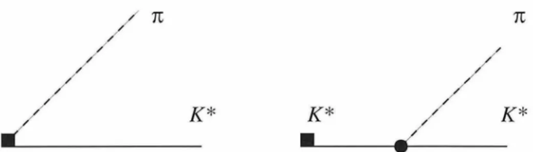
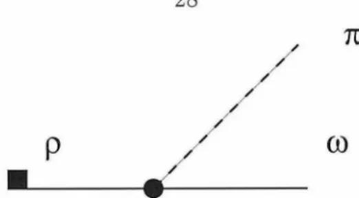
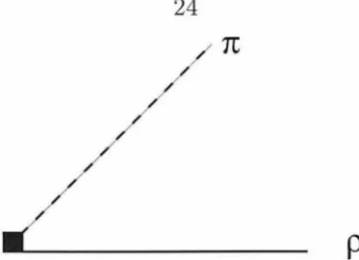
Using both heavy vector meson chiral perturbation theory and the large Ne limit, the amplitude for T ---+ W7fV7 follows from the Feynman diagram for vacuum to w7f matrix element of the left-handed current in Fig. T --+ K *nv7 falls in the kinematic region where chiral perturbation theory is valid at a T-charm or B factory [21]. Using both heavy vector meson chiral perturbation theory and the large Ne limit, we predicted the differential decay rate for T --+ wnv7 in the kinematic region where the pion is soft in the wrest frame.
We applied chiral perturbation theory of heavy vector mesons to the decay of T and used data on T --+ wnv7 to determine the magnitude of the 92 coupling in the chiral Lagrangian. For example, chiral perturbation theory of heavy vector mesons can be used to predict differential decay rates for D --+ K*7re+ve in kinematics. In this case, we combine the theory of chiral perturbations for hadrons containing heavy quarks [7] with the theory of chiral perturbations of heavy vector mesons.
- Introduction
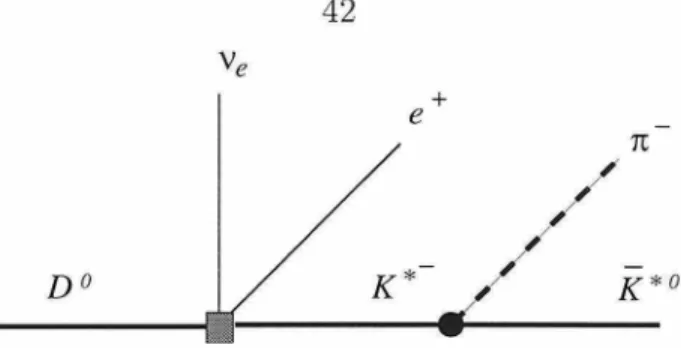
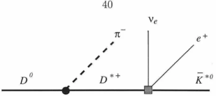
- Chiral Perturbation Theory for D 0 --+ K* 0 1f-e+ve
- Currents and the Amplitude
- Differential Decay Rate
- Summary and Remarks
The only effect of the term in Eq. 6 is thus considered the derivative of order one and has a leading order contribution in our subsequent calculations. We note that of the non-leading diagrams there are two that are not immediately seen as higher order in our chiral perturbation expansion. To make a singlet of the H, R~ and ~ fields we need a 3μ~ in the hadronic current expression.
Note that the sign of g depends on the convention for the sign of the Levi-Civita tensor, which we take to be Eµv>.rr = -Eµv>.rr = 1. Later we will only consider the region of phase space where K *0 is almost at rest in the decaying D0 rest frame and the dependence of. However, for the rest of this chapter we work in the kinematic regime where K*0 is at rest, to leading order in our calculations, in the rest frame of the decaying D0. Pe is the four-momentum of the positron, and Pv is the four-momentum of the electron neutrino.
The possibility of making such comparisons between experimental data and our theory depends on the availability and resolution of the data in the limited phase space region of our calculations. The quantities p · p7r/mD and l iJil depend on the values of the variables x, mev and cos BI<, as shown in the appendix. Let's take 9b = 0.3 to get some estimates on the magnitude of the branching ratio in our region of phase space.
We have treated D, D* and K* as heavy matter fields and applied the chiral perturbation theory formalism to describe the strong couplings of 7f- to D, D* and K*, assuming that 7f- is "soft" in the remaining frames of heavy matter fields. However, we have restricted our phase space to a region where !?*0 is close to zero recoil in the rest frame D0, making the amplitude dependence on a(-) negligible, to leading order. To obtain the branching ratio in this region, a reasonable choice must be made for the integration limits that give the fractional width in the finite volume of the phase space.
For a rough extraction of the value of gD from the experiment, we can choose an integration region where the branching ratio is of the order of 10-5. The amount of phase space where our theory is valid can best be chosen after consulting the data. Our results represent the predictions of SU(2)L x SU(2)R chiral perturbation theory at the level of one derivative, corresponding to O(vH · Pn/lGeV), where VH is the four-velocity of D0 or k0* .
Appendix
Chapter 5 Non-linear Sigma Model Solutions for the Disoriented Chiral
- Introduction
- The Non-linear Sigma Model at O(p 4 )
- The O(p 2 ) Solutions
- The O(p 4 ) Solutions
- Summary and Remarks
In the next section, we describe the nonlinear sigma model formalism in O(p4). In this chapter, we are only interested in the classical behavior of the pion field, so we do not consider loop effects. This does not mean that we can trust the qualitative behavior of solutions for arbitrarily small T.
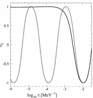
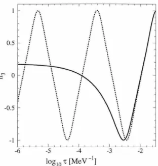
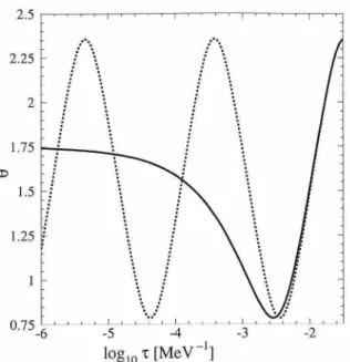
In this way, the solutions of the O(p2) equations have final values at T1. 1) to (6) we present our numerical solutions for the fields e and n and their derivatives. Note that as a result of the current conservation relations [46], n1 = 0 and n~ = 0, as in the case of the leading order solutions. The O(p2) solutions are obtained numerically and correspond to those of the analytical expressions in Eq.
In this case, we get p = 0, which is consistent with the rv ln( TI i) solution of the equation. Thus, it is the magnitudes of the derivatives that determine the region of validity of the solutions. Therefore, our results suggest that O(p4) solutions can be used to study the qualitative evolution of DCC up to a length scale of rv 0.2 fm, but O(p2) solutions lose their quality.
Therefore, the absence of the mass terms, which are important only for T ~ 1/m'Tr, does not introduce significant qualitative changes in the early real time solutions. We presented a qualitative explanation of the behavior of the solutions by studying the equations of motion in a special case and in the limit where T ~ 0. A measure of the validity of our derivative expansion is the magnitude of field derivatives.
Chapter 6 Conclusion
In Chapter 5, we presented boost-invariant (1+1) dimensional solutions for DCC, obtained numerically using the nonlinear sigma model for pion interactions at O(p4). We investigated the early correct time behavior of the solutions for which we ignored the mass terms in the Lagrangian. We noted that our O(p4) solutions could be used to present the qualitative behavior of DCC over a length scale of about 0.2 fm corresponding to a momentum scale of about 1 GeV.
Since the chiral expansion breaks down below this length scale, we found that going to higher levels in chiral perturbation theory would not allow studying DCC on smaller length scales within the nonlinear sigma model. The applications of chiral symmetry in the study of low-energy hadronic processes are many and varied. In this work, our goal was to present some applications of chiral perturbation theory and to demonstrate the power and generality of the concepts introduced in Chapter 2.
It is the author's hope that this work has achieved the above goal to some extent.
Bibliography