Arch Dams

The non-uniform motions of the foundation interface in the free field are assumed to be due to incident plane body waves. First, the free-field motion of the canyon walls is obtained by the direct boundary element method under some simplifying assumptions about the canyon geometry and earthquake mechanism. In the second part of the analysis, the frequency domain response of the dam-water-foundation system is calculated using the finite element method using previously determined free field extracts.

Details of the finite element analysis of the dam-water foundation system are presented in Chapter 2.

Chapter 2

Basic Equations

The requirements for problem 1, that the foundation interface of the structure moves with free field motion, can be met in an infinite number of ways. The dynamic component of the dam response is generated by removing the applied forces in the pseudo-static solution. The Fourier components of the dam response are obtained by superimposing pseudo-static and dynamic solutions.

Removing the forces {f5(w)} from the dam-water-foundation system results in the dynamic response {uD(w)} of the dam from the solution.

Free-field Motions

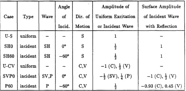
The augmented mass matrix [M(w)] is calculated directly for the generalized coordinates. horizontal free surface) due to the incident wave in the calibration half-space. For the results presented in Chapter 4, six excitations were used as listed in Table 2.1: three for the flow motion (U-S, SHO and SH60) and three for the transverse vertical motion (U-CV, SVPO and P60) where the vertical motion is approximately half that of the intersection. A single ground motion specification (scaled in amplitude according to the factors given in the table) is used for all current motions, horizontal and vertical components of the U-CV case, P and SV waves in the SVPO case, and P waves in the P60.

With reference to the calibration half-space, it would have been desirable to give different frequency contents to the horizontal and vertical components of motion, but this is not possible for an excitation like P60, where a single incident wave produces both components, so no differences were used.

Time domain results

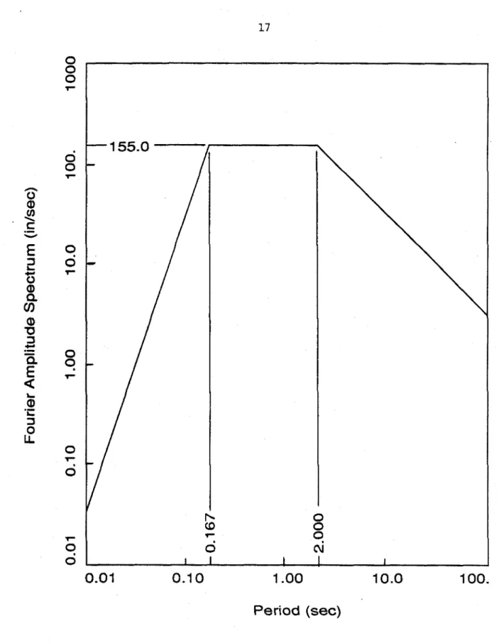
To add earthquake-like frequency characteristics to the excitation, S(w) is considered to be proportional to IF(w)l2, where IF(w)l is the modulus of the mean Fourier transform of the horizontal ground motion on a scale near a magnitude 7.5 earthquake, as is taken from [37] (Figure 2.4). The function IF(w)l represents the frequency distribution of the excitation (incident SH, P, SV waves or uniform movements in the free field); for the horizontal and vertical components of the excitation there is no difference other than the amplitude as indicated in Sect where C = constant of proportionality between S(w) and IF(w)l2 and is taken as (2.26) where Teq is the duration of seismic motion. Surface Angle Amplitude Amplitude Case Type Val Dir. of uniform excitation of the incident wave.

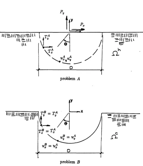
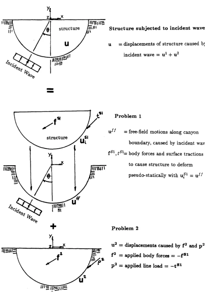
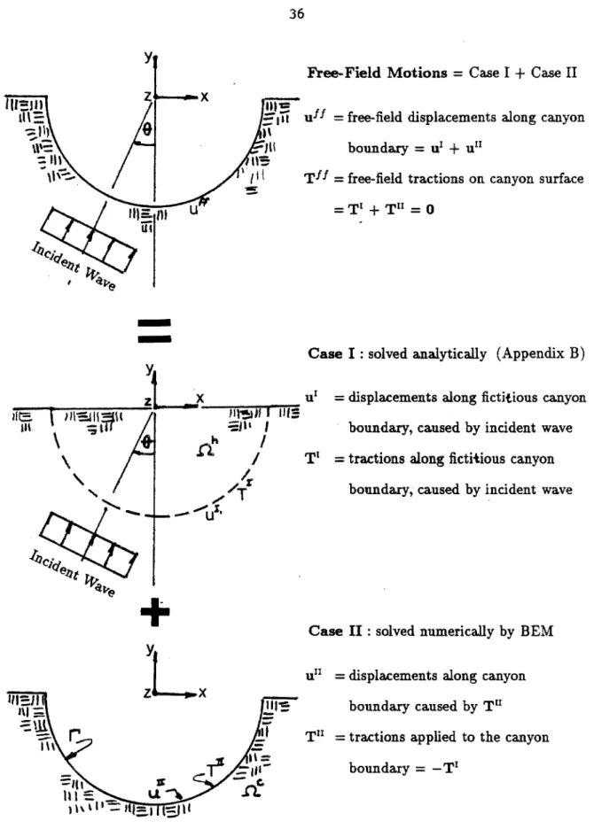
Structure subject to incident waves. u = displacements of structure caused by incident wave = u1 + u2. uf I = free field motions along the boundary of the canyon, caused by incident wave f51, t51 = body forces and surface tractions. to deform the structure pseudostatically with uf1 = uf f. u2 =displacements caused by f2 and p2 f2 =applied body forces= -fSl.

Table 2.1 : Input excitations for Pacoima dam

Chapter 3

Solution of the Free-Field Motions

Superposition Problem

Basic Equations (case II)

To form the limit integral equation, the weighted remainder method and Green's theorem are applied (twice) to the equations of motion. The weighting functions, Wr, Wy, W.~~, in the weighted remainder method have been chosen to satisfy. The above weighting functions can be thought of as displacements resulting from the Dirac delta functions, which can be interpreted as line loads or sources.

The above formulations are just statements of the reciprocal theorem and involve the solution of the case II problem in nc as one set of loads and displacements, and the solution in nh for the line sources as the other set of loads and displacements.

Solution of the Source Problem

The upper integration limit, f3ma:z:', is chosen to produce negligible clipping error and is chosen to be that given by a transform wavelength equal to 1/6 the sum of the source point depth and the response depth. point;. A/3 first exceeds [21r /10K6(x- x 6)]), the integrand is approximated as a square over each pair of A/3 using three sampling points and integrated analytically. This part of the integral is evaluated as the Cauchy principal value and includes the remainder of the integrand at the pole.

Therefore, the cos or sin term is separated and analytically integrated with the remaining integrand, which is approximated as a quadratic (again using three sampling points for each 6./3 pair).

Solution of the Integral Equation

Four procedures are needed, depending on whether the integrand contains the ukTf1 term or the Tkur term, k = x, y, z, and whether node s is at the top of the gap on the horizontal free surface (nodes 1 and n, figure 3.6) or below the horizontal free surface. The Hankel functions contained in the line source displacements (Appendix C) are expressed as the sum of single terms (ln(rs) and for the plane strain displacements, 1/rs) and a series of non-singular terms (2), and are combined according to the expressions in the appendix Extension of the Hankel functions in the line load tractions along r-fE, and combination according to the expressions in appendix C yields Tk = st + ns, where st = constant times (l/rs ) (independent of w ).

Forst x 1, however, the singular term constants for two adjacent elements are equal but opposite in sign, so that there is no contribution except at the end of the longer element if the adjacent elements differ in length.

Comparison with Previous Solutions

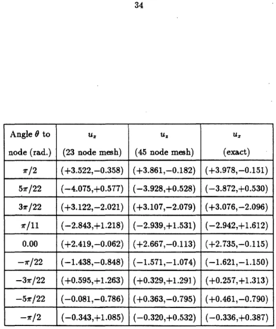
In addition to the above checks on the plane strain problem, three other tests were performed. The accuracy of the boundary element values (exact values from [41]) was similar to that obtained in the SH verification study. Since this test problem did not exercise parts of the boundary element program dealing with the horizontal surface of the half-space, in particular the inverse Fourier transform, this part of the program was separated and used to solve the problem of a uniformly distributed load on the surface of a half-space between x = ±b.

The third test problem (Figure 3.9) simultaneously exercised most of the program and used a set of pulls rr, k = x, y applied to a semicircular canyon in a half-space.

Artificial Resonances

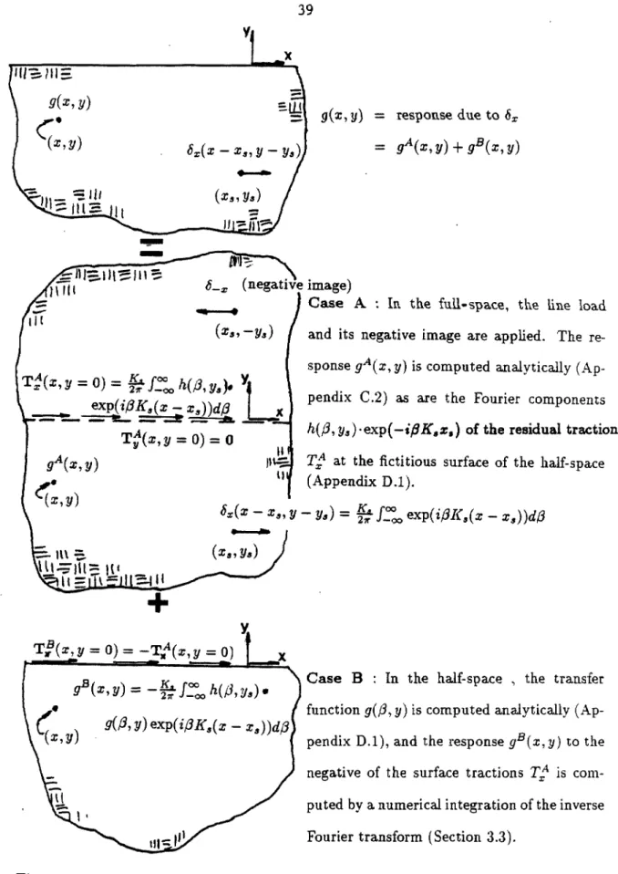
In terms of equation 3.21, involving integration over r-P, only the cos(jO) component of the traction Tz and the displacement Uz due to the line source will contribute; so one has only to consider. A more general treatment would reveal that the degeneracy occurs in the planar strain problem... and for arbitrary canyon geometries, but not for the solution of the internal problem and not for source applications away from the canyon boundary r. The response gA(x,y) is calculated analytically (Appendix C.2), as are the Fourier components h(j3,y,)·exp(-i{3K.z,) of the residual traction.

Example B : In the half-space, the transfer function g(j3,y) is calculated analytically (Appendix D.l), and the response gB(x,y) to the negative surface force TxA is calculated by numerical integration of the inverse Fourier transform (Section 3.3).

Table 3.1 : Displacements (real pa.rt, imaginary part) for a. horizontally incident (0 = 90°) SH wave on a semicircular canyon ('1/Js = 4.0)

Results of Analysis of Pacoima Dam Subjected to Uniform and Nonuniform Seismic Input

Free-Field Motions

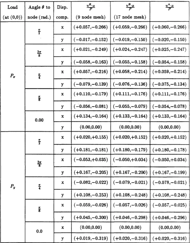
The last column of the table gives the sum of incident and reflected amplitudes on a horizontal, free surface; thus the first three cases (current excitation) are consistent and the last three cases (C-V excitation) are about the same. With this reference, amplitudes of the current, cross-current and vertical motion components are approx. 1, 1, and t, respectively. Free-field motions of Pacoima canyon for the excitations listed in Table 2.1 were calculated between 0.0 Hz.

7 on one bank to 0.3 on the other with a phase difference of about 0.4 cycles (Figure 4.3e), compared to an in-phase motion of amplitude 1.0 for the uniform excitation. Much of the increase is due to the integration required by the inverse Fourier transforms.

Discretization of Pacoima Dam, Foundation and Reser-

Results of Analysis

As discussed in Chapter 2, the calculations use eigenvectors of the dam foundation system as general coordinates. The pseudo-static component of the response is largest near the perimeter of the dam, where it can be a significant fraction of the total response. This fraction is small in the interior of the dam except for the stresses at low frequencies, where.

Thus, the importance of the pseudo-static voltages can only be quantified in the time domain when specifying the low-frequency content of the motion. Other quantification of the effect of non-uniform seismic input can be obtained in the time domain. Each figure contains six parts (one for each of the excitations in Table 2.1), and each part contains four.

Time domain quantification of the pseudo-static component of the response shows that it is small, only reaching the 27% level at the ends of the upper arc (Figures 4.12e and 4.13e). In general, the largest pseudo-static stresses occur near the foundation interface, where the dynamic component of the response (total minus pseudo-static) is small. The increase in amplitude of the fundamental symmetric resonance for P60 excitation is strongly displayed.

The responses in Figures 4.12 and 4.13 are only relative values and as such are independent of the constant C in Equation 2.25. From equation 2.26, choosing the duration Teq allows obtaining the actual responses to the input from figure 2.4.

Table 4.1 : Average of standard deviations of total arch stress along the crest expressed as a percent of the average for excitation U-S with a full reservoir

CIJ CIJ

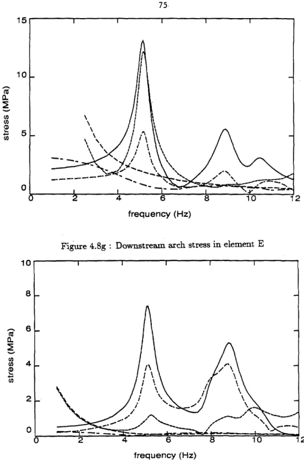
Downstream arc voltage in element B Figure 4.10g Downstream arc voltage in element E Figure 4.10h Downstream cantilever voltage in element C Figure 4.10i.

Figure 4.8g: Downstream arch stress in element E

0.. CIS

Chapter 5

Conclusions and Recommendations for Future Work

Conclusions

Future Work

When the earthquake excitation is perpendicular to the flow direction, current design methods may overestimate or underestimate the actual stresses within the dam. The free-field motions generated by the present technique can also be used in the seismic analysis of long-span bridges over deep canyons.

Seismic analysis of arch dams, including dam-water interaction, reservoir boundary absorption, and foundation flexibility. Dynamic and seismic behavior of concrete dams: a review of experimental behavior and observational evidence.

Appendix A

Notation for Appendices

Appendix B