Odds Ratio Methods for Unstratified Closed Cohort Data 89 4.1 Asymptotic Unconditional Methods for a Single 2×2 Table, 90 4.2 Exact Conditional Methods for a Single 2×2 Table, 101 4.3 Asymptotic Conditional Methods for a Single 2×2 Table, 406' Cornfields. Approximation, 109. Hazard ratio methods for closed cohort data 143 6.1 Asymptotic unconditional methods for a single 2×2 table, 143 6.2 Asymptotic unconditional methods forJ(2×2) tables, 145 6.3 Mantel–Haenszel estimate of, R148 estimate.
PROBABILITY
Probability Functions and Random Variables
For the present discussion we assume that the sample space of the joint probability function is the set of pairs {(x,y)}, where is in the sample space of XandY in the sample space of Y. We say that XandY are independent random variables ifP( X =x,Y =y)=P(X =x)P(Y =y), so if the joint probability function is a product of the marginal probability functions.
Some Probability Functions
In fact, the Poisson distribution can be derived as a limiting case of the binomial distribution. As can be seen, the Poisson distribution provides a progressively better approximation to the binomial distribution as π gets smaller.
Central Limit Theorem and Normal Approximations
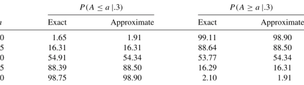
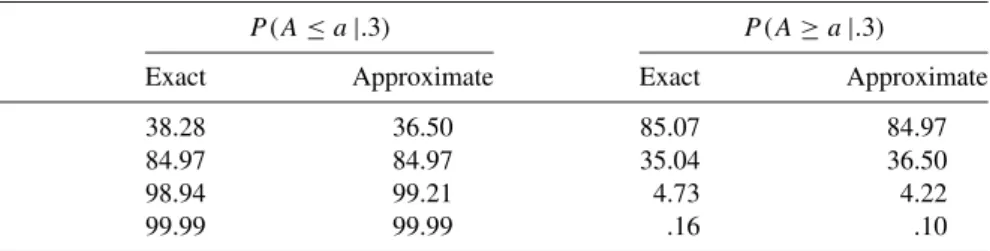
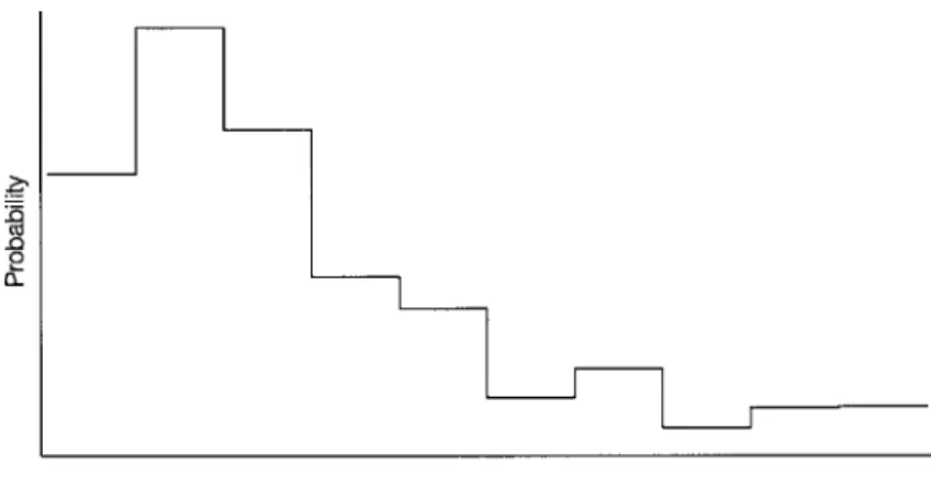
Example 1.6 Table 1.6(a) gives the exact and estimated values of the lower and upper tail probabilities of the binomial distribution with parameters (.3,10). The horizontal axes are labeled with the term "count", which represents the number of binomial or Poisson outcomes.
PARAMETER ESTIMATION
Maximum Likelihood
We refer to this value of θ as the maximum likelihood estimate and denote it by θ.ˆ. It seems that the maximum likelihood method has a lot to offer; however, there are two potential problems.
Weighted Least Squares
It is easy to show that the maximum likelihood equation (1.17) simplifies to a− ˆπr =0 and thus the maximum likelihood estimate is πˆ =a/r. First, the maximum likelihood equation can be very complex and this can make the calculation of θˆ difficult in practice.
RANDOM SAMPLING
Simple Random Sampling
To enable stratified random sampling, it is necessary to know in advance the number of individuals in the population in each stratum. Most procedures in standard statistical packages, such as SAS (1987) and SPSS (1993), assume that data has been collected using simple random sampling or stratified random sampling.
SYSTEMATIC AND RANDOM ERROR
Since the coin is fair, based on the binomial model, the probability of observing the data in the second replicate is 100. In the current example, the null hypothesis would be that the chemical is not associated with cancer risk.
MEASURES OF EFFECT
Closed Cohort Study
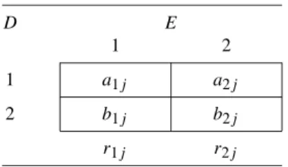
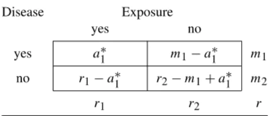
In a closed cohort study involving a single sample, the parameter of interest is usually the binomial probability of developing the disease. Consider a closed-group study in which exposure is dichotomous and assume that at the beginning of the follow-up there are r2 subjects in the exposed group (E=1) and r2 subjects in the unexposed group (E =2).
Risk Difference, Risk Ratio, and Odds Ratio
Since ω1=ORω2, the odds ratio is similar to the hazard ratio in that the difference is measured on a multiplicative scale. In some of the older epidemiological literature, the odds ratio was seen as little more than an approximation of the hazard ratio.
Choosing a Measure of Effect
It also illustrates that the risk difference and risk ratio have a straightforward and intuitive interpretation, a feature not shared by the odds ratio. It appears that, from the point of view of ease of interpretation, the risk difference and the risk ratio have a distinct advantage over the odds ratio.
CONFOUNDING
Counterfactuals, Causality, and Risk Factors
Sometimes the definition of what constitutes a risk factor is expanded to include characteristics that are closely related to a causal agent but not necessarily causal in themselves. In this sense, carrying a lighter can be considered a risk factor for lung cancer.
The Concept of Confounding
So after accounting (controlling, adjusting) for smoking, we conclude that drinking is not a risk factor for this disease. In the crude (unstratified) analysis, drinking appears to be a risk factor for lung cancer due to what we will later refer to as confounding by smoking.
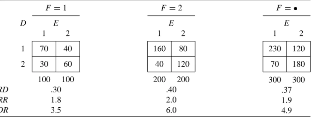
Some Hypothetical Examples of Closed Cohort Studies
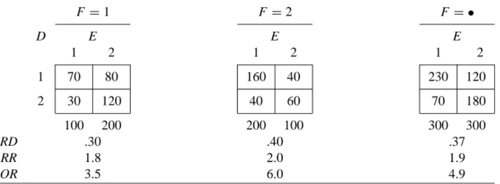
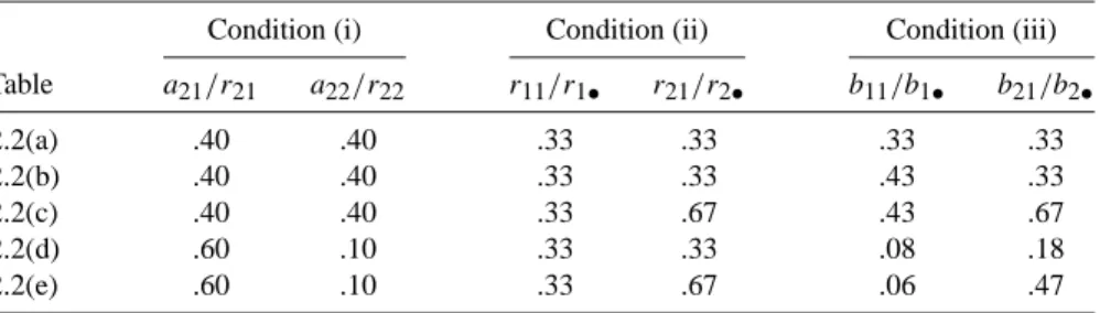
In Table 2.2(a), for each effect measure, the stratum-specific values are equal to each other and to the crude value. When some or all of the stratum-specific values of the effect measure differ (across F strata), this phenomenon is described by any of the following synonymous terms: The effect measure is heterogeneous (across F strata).
COLLAPSIBILITY APPROACH TO CONFOUNDING
- Averageability and Strict Collapsibility in Closed Cohort Studies In this section we carry out an analysis of the risk difference, risk ratio, and odds ratio
- Risk Difference
- Risk Ratio
- Odds Ratio
- A Peculiar Property of the Odds Ratio
- Averageability in the Hypothetical Examples of Closed Cohort Studies We showed at the beginning of Section 2.4.1 that if a measure of effect is averageable,
- Collapsibility Definition of Confounding in Closed Cohort Studies We are now in a position to describe and critique the collapsibility definition of
For now, we also assume that F is not an effect modifier of the risk difference. For example, in Table 2.2(d), F is a confounder of the odds ratio, but not the risk difference.
COUNTERFACTUAL APPROACH TO CONFOUNDING
- Counterfactual Definition of Confounding in Closed Cohort Studies In Section 2.3.1 we introduced the idea of counterfactual arguments in discussions
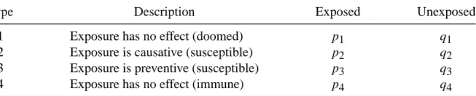
- A Model of Population Risk
- Counterfactual Definition of a Confounder
- Standardized Measures of Effect
The risk difference would be unreasonable provided that the probability of death in this comparison group was equal to the probability of death in the unexposed counterfactual group. This avoids the problem associated with the likelihood ratio that was identified as a flaw in the definition of confounding.
METHODS TO CONTROL CONFOUNDING
There is evidence in the UGDP data (not shown) that variables other than age were unevenly distributed in the two treatment arms. Nevertheless, stratification is almost always used in the exploratory stages of an epidemiological data analysis.
BIAS DUE TO AN UNKNOWN CONFOUNDER
A problem with this approach is that the data may not accurately reflect the situation in the population as a result of random and systematic errors. As can be seen, provided that the unknown confounder has a low prevalence in the unexposed population, is not closely related to exposure, and is not a major risk factor.
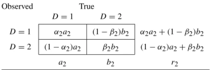
MISCLASSIFICATION
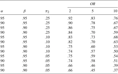
This indicates that, provided α+β >1, nondifferential misclassification biases the observed odds ratio toward “zero”—that is, toward 1 (Copeland et al., 1977). When the exposure variable is polychotomous—that is, it has more than two categories—observed odds ratios may skew toward zero or may even have values on the other side of zero (Dosemeci et al., 1990; Birkett, 1992).
SCOPE OF THIS BOOK
When this occurs, odds ratios may deviate from the null value, spurious heterogeneity may appear, and true heterogeneity may be masked (Greenland, 1980; Brenner, 1993). One of the goals of this book is to identify a select number of non-regression techniques that are computationally convenient and can be used to explore epidemiological data prior to more detailed regression analysis.
EXACT METHODS
Hypothesis Test
To calculate the two-sided p-value we need a method to determine a corresponding probability on the "other side" of the distribution. One possibility is to define the second probability as the largest tail probability on the other side of the distribution that does not exceed pmin.
A Critique of p-values and Hypothesis Tests
Given these uncertainties, in epidemiology we are usually interested not only in whether the true value of a parameter is equal to some assumed value, but, more importantly, what is the range of plausible values for the parameter. In recent years, the epidemiological literature has become critical of p-values and has placed increasing emphasis on the use of confidence intervals (Rothman, 1978; Gardner and Altman, 1986; Poole, 1987).
Confidence Interval
Since an exact confidence interval is obtained by inverting an exact test, when the distribution is discrete, the resulting exact confidence interval will be conservative—that is, wider than indicated by the nominal value of α (Armitage and Berry, 1994 , p. 123). Note that the confidence interval includes π0=.4, a finding that is consistent with the results of Example 3.1.
ASYMPTOTIC METHODS
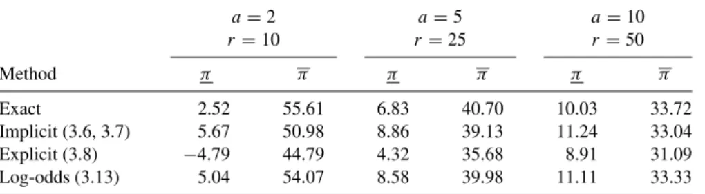
No Transformation Point Estimate
We will call this the implicit confidence interval estimation method because π and π are present in the variance terms (3.6) and (3.7). An alternative approach, which we call the explicit method, is to replace π and π in the variance expressions with the point estimate πˆ =a/r.
Odds and Log-Odds Transformations Point Estimate
In this chapter we discuss odds ratio methods for analyzing data from a closed cohort study (Section 2.2.1). Compared to the risk ratio and risk difference, however, it is true that methods based on the odds ratio are more easily applied to other epidemiological study designs.
ASYMPTOTIC UNCONDITIONAL METHODS FOR A SINGLE 2 × 2 TABLE
Case 4.2 (receptor level – breast cancer) Data for this case were kindly provided by the Northern Alberta Breast Cancer Registry. Returning to the analysis of the data in Table 4.5(a), the expected numbers given in Table 4.6 are much greater than 5.
EXACT CONDITIONAL METHODS FOR A SINGLE 2 × 2 TABLE The methods presented in the preceding section are computationally convenient but
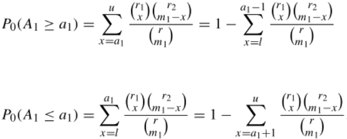
A convenient method for tabulating a central hypergeometric probability function is to form each of the possible 2×2 tables and compute probability elements using (4.16). Calculation of the two-tailed p-value using the cumulative or doubling method follows exactly the steps described for the binomial distribution in section 3.1.1.
ASYMPTOTIC CONDITIONAL METHODS FOR A SINGLE 2 × 2 TABLE
Conditional asymptotic methods make it possible to reduce the computational burden, at least in the case of the link test. For the conditional asymptotic analysis we consider (4.13) as a probability that is a function of the parameter OR.
CORNFIELD’S APPROXIMATION
Example 4.7 (Antibody–Diarrhea) For the antibody–diarrhea data, the estimated odds ratio is ORc=7.17, which is obtained by solving. Once determined, the remaining entries in the cells are determined as in Table 4.12, thus ensuring that the estimated calculations match the initial marginal totals.
SUMMARY OF EXAMPLES AND RECOMMENDATIONS
ASYMPTOTIC METHODS FOR A SINGLE 2 × I TABLE
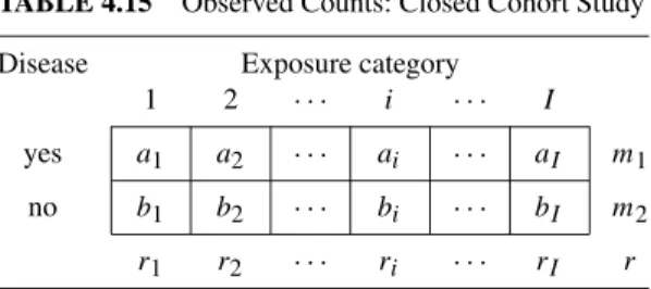
When the null hypothesis is rejected by one of the above tests, the interpretation is that overall there is evidence for a connection between exposure and disease. For a continuous exposure variable, a reasonable approach is to define the exposure level for each category to be the midpoint of the corresponding cutpoints.
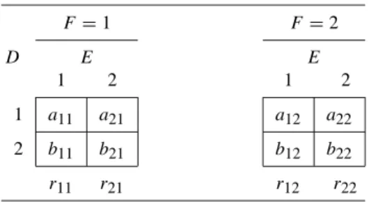
Each of the tables can be analyzed separately using the methods of Chapter 4. The layer-specific estimates are. From Example 4.2, the crude odds ratio estimate of the association between receptor level and breast cancer survival is ORu =3.35 and the 95% confidence interval for ORis.
Also, (4.28) and (5.8) relate the fitted counts based on the asymptotic unconditional and asymptotic conditional methods. Comparing Tables 5.5 and 5.7, the fitted counts based on the asymptotic unconditional and asymptotic conditional methods are almost identical.
MANTEL–HAENSZEL ESTIMATE OF THE ODDS RATIO
Before (5.31) became available, the test-based method of estimating var(logORmh) was commonly used. The test-based approach "solves" this equation forvar0(logORmh) and defines the estimate of var(logORmh) to be.
The second term in (5.32), which comes from Tarone (1985), corrects for the use of ORmh instead of the more efficient estimate ORu. Liang and Self (1985) and Liang (1987) describe tests of homogeneity for the sparse-strata setting, but the formulas are complicated and will not be presented here.
INTERPRETATION UNDER HETEROGENEITY
Even when some of the terms are quite large in absolute value, Xmh2 can be small due to the cancellation of positive and negative terms. For this reason, it is prudent to establish homogeneity before conducting an association test.
In the latter case, there may be significant associations in some strata that were not detected by the general test. The local property of Xt2 means that it is not sensitive to misspecification of the exposure–disease relationship model.
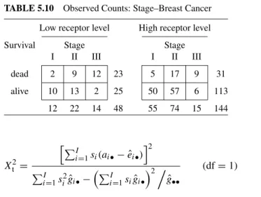
Example 5.5 (stage breast cancer) Table 5.10 shows the observed numbers corresponding to table 4.16 after stratification by receptor level. Arguing along the lines of Example 5.1, a rationale can be provided for treating receptor level as a confounder of the association between disease stage and breast cancer survival.
ASYMPTOTIC UNCONDITIONAL METHODS FOR A SINGLE 2 × 2 TABLE
Hazard ratio methods for analyzing closed cohort data have many similarities to the odds ratio methods in Chapters 4 and 5. However, hazard ratio methods based on asymptotic unconditional, Mantel-Haenszel, and weighted least squares methods are available for analyzing closed cohort data. .
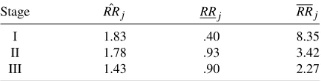
It is interesting that, unlike Table 5.4 where the odds ratio estimates have an increasing trend, the risk ratio estimates show a decreasing trend. Recalling the results of Example 5.1, the data in Table 5.3 appear to be homogeneous with respect to both the odds ratio and the risk ratio.
MANTEL–HAENSZEL ESTIMATE OF THE RISK RATIO
As noted in Section 5.6, tests of homogeneity generally have low power and, as such, may fail to detect heterogeneity even when it is present. Thus, one explanation for the previous contradictory finding is that one or both of the odds ratio and the hazard ratio are actually heterogeneous, but this was not detected by the homogeneity tests.
SUMMARY OF EXAMPLES AND RECOMMENDATIONS
Risk difference methods for analyzing closed cohort data are similar to those based on the hazard ratio.
ASYMPTOTIC UNCONDITIONAL METHODS FOR A SINGLE 2 × 2 TABLE
In fact, the previous chapter and the current one have so much in common that it is possible to use here language almost identical to that of Chapter 6. Note that (7.2) is precisely the variance estimate that results from applying ( 1.9). to the random variableπˆ1− ˆπ2.
The data for this example is taken from Table 4.5(a). the methods of the previous section. Probability Ratio Test of Homogeneity The probability ratio test of homogeneity is. df=J−1) which is identical in form to (5.18) but uses adjusted counts based on the risk difference.
MANTEL–HAENSZEL ESTIMATE OF THE RISK DIFFERENCE The Mantel–Haenszel estimate of the risk difference is
The 95% confidence intervals are quite wide, and each contains estimates of risk differences for the other two strata, suggesting the presence of homogeneity. Comparing the fitted counts in Tables 5.5, 6.2 and 7.2 with the observed counts in Table 5.3, there appears to be little to choose between the odds ratio, risk ratio and risk difference models in terms of goodness of fit.
SUMMARY OF EXAMPLES AND RECOMMENDATIONS
There are more general methods for analyzing group data, which are collectively referred to as survival analysis. In this chapter we will discuss some of the basic ideas in survival analysis such as censoring, survival functions, hazard functions, proportional hazards assumption, and competing hazards.
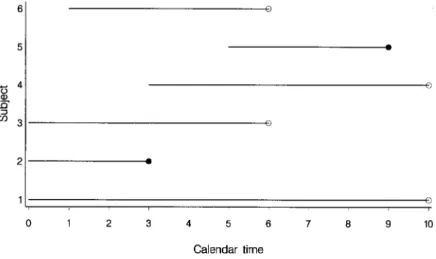
OPEN COHORT STUDIES AND CENSORING
This results in Figure 8.1(b), in which all trace lines have been given the same origin. Now consider a person who is censored because he was lost to follow-up after moving out of the study area.
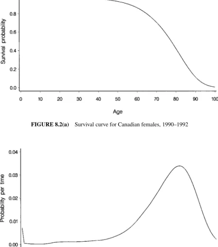
SURVIVAL FUNCTIONS AND HAZARD FUNCTIONS
In Figure 8.2(c), the hazard function shows the same patterns observed in the survival function and probability function. In particular, we see the rapid increase in the hazard function as the extreme age approaches.
HAZARD RATIO
In the epidemiological literature, the hazard ratio is sometimes referred to as the incidence density ratio. It is important to appreciate that the proportional hazards assumption specifies that the ratio of the hazard functions is constant, not the individual hazard functions.
COMPETING RISKS
In the statistical literature, hk(t) is referred to as the raw hazard function for causek (Chiang, 1968, Chapter 11; Elandt-Johnson and Johnson, 1980, Chapter 9; Tsiatis, 1998). In this case, we drop the term "in the presence of other causes of death" from the previous interpretation and refer to tohk(t) as the net hazard function of causek (Chiang, 1968, Chapter 11; Elandt-Johnson and Johnson, 1980, Chapter 9; Tsiatis, 1998 ).
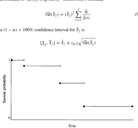
KAPLAN–MEIER SURVIVAL CURVE
In the case of the Kaplan–Meier method, nothing is assumed about the functional form of either the survival curve or the hazard function. In fact, another name for the Kaplan–Meier approach to censored survival data is the product-limit method.
ODDS RATIO METHODS FOR CENSORED SURVIVAL DATA
- Methods for J (2 × 2) Tables
- Assessment of the Proportional Hazards Assumption Graphical Method
- Methods for J (2 × I) Tables
- Adjustment for Confounding
- Recommendations
Example 9.3 (Receptor Level-Breast Cancer) Figure 9.3(b) is taken directly from Figure 9.3(a) by applying the log-minus-log transformation. In the previous analysis, we treated stage as a confounder of the risk association between receptor level and breast cancer survival.
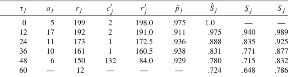
ACTUARIAL METHOD
The actuarial approach to estimating the survival function continues along the lines of the Kaplan-Meier method. Since so little structure is imposed, it is convenient to view a Kaplan-Meier survival curve as a kind of scatterplot of censored survival data.
POISSON METHODS FOR SINGLE SAMPLE SURVIVAL DATA In theory, a hazard function can have almost any functional form. The estimated
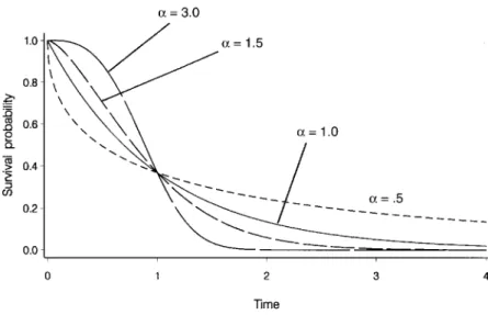
Weibull and Exponential Distributions
The exponential distribution is based on the assumption that the hazard function is constant over the entire follow-up period. The attractive thing about the exponential distribution is that the parameter λ can be easily estimated, as shown below.