The measurement of the total charged current cross-section for neutrinos and antineutrinos on iron is described. Two years later, Fermi came up with a quantitative description of the weak interaction [FE34].

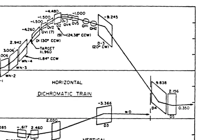
Principles of the Di.chromatic Neutrino Beam
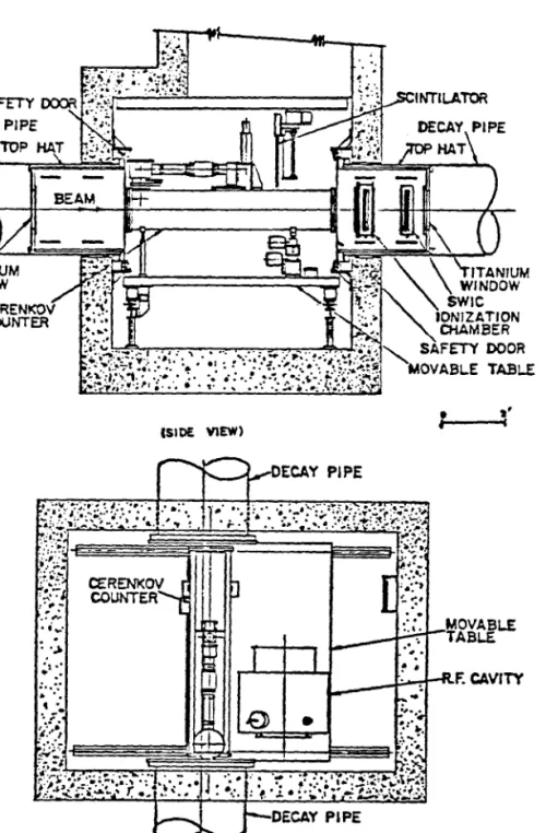
The smooth curves are from the ideal radius calculation {see text). points with horizontal error bars span a realistic beam phase space. At the end of the decay pipe is a 20-foot steel and aluminum dump to stop the secondaries.

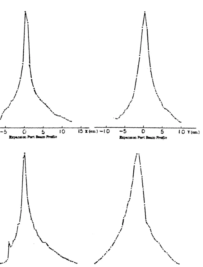
Total Secondary Flux Measurement
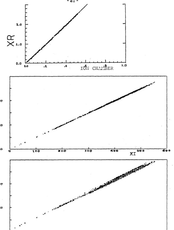
We can then compare the output of the ion chamber in pico Coulombs to the RF output. Another method used to calibrate the ion chamber was to introduce main ring protons through the train and use the sheet radiation to determine the relative intensity before and after the train.
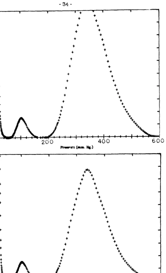
Cherenkov Counter Pressure Curves
- Electron and Muon Content of the Beam
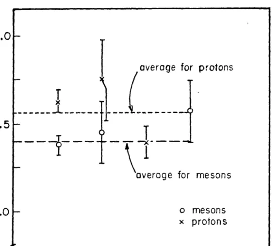
- Average Momentum
This background was only significant in the low-pressure portion of the Cherenkov curve (see Figure 2-13). The position of the peak in the Cherenkov curve for such a radius and the iris dimensions.

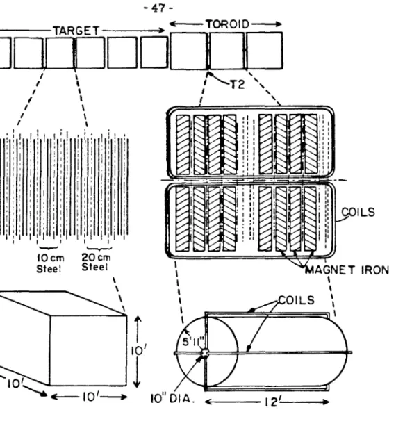
Target Statistics and Layout
- Muon momentum resolution
Both the target and the toroidal magnet are sandwiches of iron, scintillation counters, and spark chambers (spacing and layout details can be found in Table 3-1 and Figure 3-1). The target was organized into six approximately cubic blocks which could be moved on track (perpendicular to the instrument axis) into the N5 charged particle beam line. This structure and the nearby charged particle beam made calibration and resolution measurements possible directly on the instrument.
For completeness, a brief description of the device is included here, but more details can be found in reference [LEB:]. There are six spark chambers in each target cart, a set of spark chambers between the toroid carts and in the opening in the center of each toroid cart. The chambers were fixed (aligned) relative to each other using muons passing through the entire device. The accuracy of this procedure was 10 mils in the target and 15 mils in the torus chambers.
The amount of steel between the chambers and the chamber resolution determine the accuracy with which a muon's momentum can be reconstructed from its toroid track. The room resolution contributes very little to this value (<1%) in the energy range of this experiment.
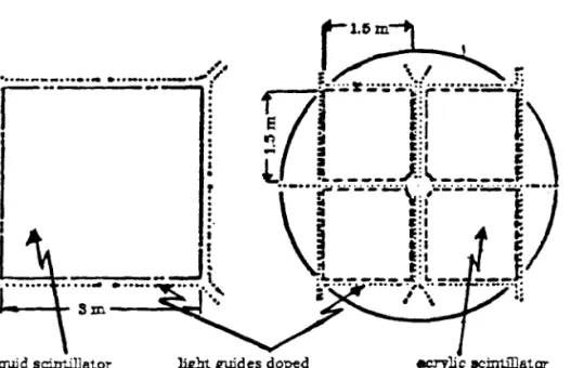
Scintillation counters
For each tube, a "low" ADC digitized the tube output, a "high" ADC digitized the output of the sum of all tubes in a counter, and a "super low" ADC digitized the output of the sum of multiple tubes in different counters. This was sufficient for all but a very small (<1%) number of events where one of the "low" ADCs was saturated, in these cases the appropriate superlow was used to recover that tube's output. The size of the target counters is on the order of the dimming length of the blue light that must travel to the edge (a 10' counter length compared to dimming lengths of about 6').
A counter response model was built which had 4 parameters, the center of the counter relative to the spark gaps and the horizontal and vertical. This model used the known optical properties of the meters to calculate (given the above parameters) the expected light output of each tube. For each neutrino interaction, we measured the event interaction point and the output of each tube.
As a check on this procedure, we took hadron beam data at various points in one of the neutrino target vehicles. In order to correct for week-to-week and month-to-month variations in counter outputs, we averaged the pulse heights of muons that traversed within 30" of the center of each counter from about 0.1 to 2 times the minimum ionizing pulse height.
Horizontal (inches)
Approximate Run Number
Counter
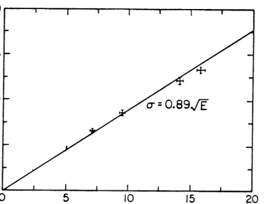
- Hadron Energy Calibration and Resolution
- Trigger Electronics
- Muon Trigger
- Penetration Trigger
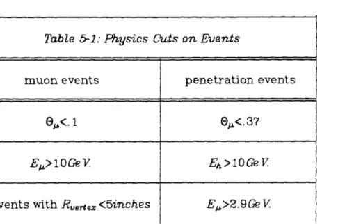
- Cuts on Events
- l. Unanalyzable events
- Events with Improper Track Reconstruction
- Monitor Cuts (applied to monitors and events)
- Ion Chamber Selection
- Cross Sections
- Method of Counting Events
Fi.Eure 3-12: The effectiveness of the muon and penetration triggers after all software tracks (see section 5.1). After subtracting cosmic rays, the last two categories account for less than 1% of the events used in the analysis. A plot of the efficiency of passing this cut versus true muon momentum as the muon enters the toroid appears in figure 4-1.
A simple parameterization of the shape of the efficiency versus Pµ of the form o:.(1+.0196(pc-1B)0(1B-p0)) was used to correct for lost muon triggers (p0 is the momentum that evaluated at the face of the first toroid). The average momentum reconstruction efficiency (after correction for the muon momentum dependence of this efficiency) is plotted for each of the 10 secondary settings. The number of nucleons per unit area was obtained by taking the known mass of the target steel (each plate was weighed before installation) and an estimate of the additional mass due to scintillation counters and chamber material (corresponding to 7% of the target mass) in the reference volume and combined with.
For muon events, the efficiency is extended to include a translation of the interaction point along the z axis. An additional correction must be made to muon events to account for those cases where the momentum of the muon cannot be determined by the fitting program.
Hadron Energy in GeV
A Monte Carlo calculation was used to adjust for the losses resulting from these cuts; the Monte Carlo corrections are listed in Table 5-2.
RADIUS (inches)
Cross Section Results
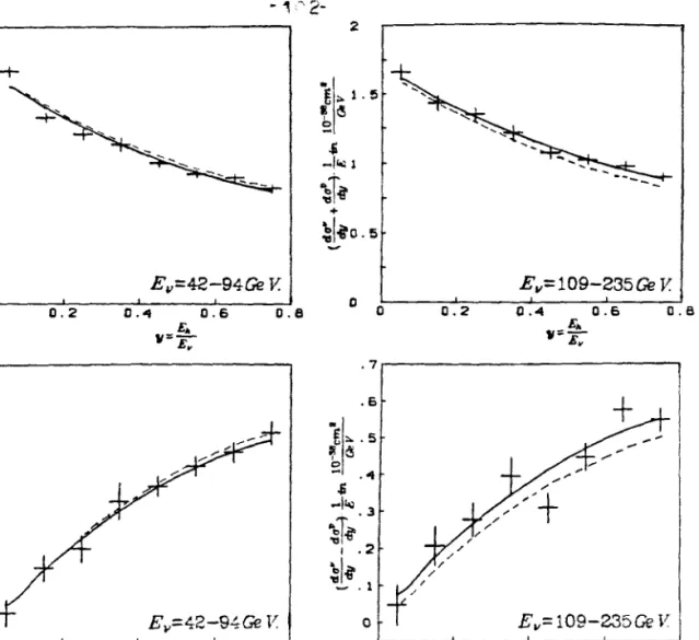
After making the cross sections for each 5" radial bin and each energy setting, the results are averaged over the energy ranges. These averaged cross sections and an indication of the range of average neutrino energy used (averaged within the 5" bin) are listed in Table 5-4 and plotted in Figure 5 -7. The data are plotted together with the assumptions that: top graph: the number of broadband events is proportional to the area from which the events are collected (dotted lines positive - dashed negative) bottom graph: the number of broadband events is proportional to the number of protons on the target regardless of setting .
The neutrino flux from kaon three-body decays is described together with the neutrino flux from two-body decays. Thble Er40: Neutrino and antineutrino cross sections. the following errors do not include a standard error of magnitude 5.9%).

- Differential cross section at y=O
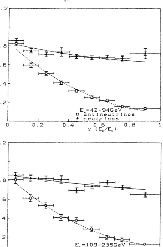
The second method is to use the properties of the dichromatic beam to predict for a given peak location in the target what the average neutrino energy is, giving y2= Ev(R). For neutrinos from pion decay the transition point was taken at y=.2 and for neutrinos from kaon decay y =.4, using these values ensured that the low y acceptance corrections were small (<3%). Fits of this form are shown in Figures 5–8, and the results of fitting pion and kaon decay neutrinos for all settings are given in Tables 5–6.
For an isoscalar target (one having an equal number of neutrons and protons) as y approaches 0 the cross section should be the same for neutrinos and antineutrinos, provided we stay well above the threshold of charming and strange particle production. The reason for this is that the sea which is invariant under CP will have the same probability for interaction with neutrinos and antineutrinos, the probability for scattering of valence quarks at y=. O is proportional to ZG:E ·
The y=O value of the fit to the y distribution is plotted for each energy setting in Figure 5-9. Using only the low y data gives fr/F2dx as described in Table 5-7, along with other measures of this quantity.
E 11 (GeV)
Average y
The average value of y is a measure of the relative amount of quark and antiquark in the nucleon. The predictions of the NQPM allow us to relate different aspects of the distributions and the cross-section. Given the assumption that deviations of the cross-sectional slope from energy independence are all caused by a W-propogator effect, the confidence level is vs.
The sum of the neutrino and antineutrino cross sections gives the average x of the valence plus sea distributions in the nucleon. The curves indicate the value of the integral of F2 over x obtained by integrating F2(x, cf) over x for the same Q2 as neutrino interactions using models of F2 derived from fits to ed(SLAC -[ABBO]) and µFe ( EMC -[AUB1]) scattering. The same quantity is measured in electron and muon scattering (modulo a factor of the mean square quark charge.
For example, if the b quark were to merge via a Cabbibo species mixing with lighter quarks, then, since muo production does not change quark flavors, it would have no effect (ie the b quark sea could be too small). A careful study of dimuon production from neutrino and muon scattering experiments may clarify this apparent discrepancy.
In GeV
Neutrino Oscillations
By far the largest uncertainties in the cross-section arise from our ignorance of the properties of the connecting beam. This part of the ionization depends on the nuclear cross-section of the particles being tracked. The calibration of the ion chamber after adjustment to zero protons is shown in Table Al-4.
The neutrino flux depends on the momentum, momentum bite and angular divergence of the secondary beam. For R< Finally, the angular distribution of the secondary should be considered as an important beam parameter. However, the opening at the end of the train serves to place a limit on the size of the beam at the start of the downpipe. The error listed is that due to the uncertainty in size at the end of the train. 25%, which is the root mean square deviation of the Monte Carlo SVNC estimate.