Using targeted short-term field investigations to calibrate and evaluate the structure of a hydrological model.
D.A.Hughes1, M. Gush2, J. Tanner1 and P.Dye3
1Institute for Water Research, Rhodes University, Grahamstown, South Africa.
2CSIR, Natural Resources & Environment, Stellenbosch, South Africa.
3University of the Witwatersrand, School of Animal, Plant & Environmental Sciences, Johannesburg, South Africa
Abstract: This study combines the application of a hydrological model with the use of field data derived from short period measurement campaigns at two sites, one a low topography forested area and the other a steep grassland catchment. The main objective was to determine if the structure of the widely-used Pitman model could be considered appropriate for simulating the field data. The model is typically applied at coarse spatial and temporal (1 month) scales, while the tests reported here use data from small catchments and are applied in a daily version of the model. The results demonstrate the importance of ensuring that field observations are measuring the same hydrological variables as the model simulations. At one study site there was a mismatch in the soil moisture data that was corrected by incorporating a 2-layer soil algorithm into the model. The model results from both field sites identified the sensitivity of the model to assumptions about evaporative demands and indicate that the model structure is very sensitive to the potential evaporation inputs. The overall conclusion is that the model structure is generally appropriate for simulating the hydrological responses at the two sites, but that there remain some unresolved uncertainties about specific model components and the use of certain types of input data. The study lends support for the future development of a more complete daily version of this widely-used model.
Key Words: Hydrological modelling, field data, forest evapotranspiraton, soil moisture, model structure.
INTRODUCTION
Hydrological models are typically calibrated or assessed using long-term observed stream flow data drawn from national gauging networks. Unfortunately, this means that the model may represent the overall response of the catchment but for the wrong reasons (Kirchner, 2006). This is particularly true for models which have relatively complex structures and many
parameters representing different catchment processes and are therefore subject to the problems of equifinality (Beven, 2006). Hughes (2010a) argued that equifinality is present in natural systems and it may be an advantage to have models that can simulate similar responses for different reasons. However, this is only true if the model equifinality can be resolved with adequate quantitative understanding of real processes (Seibert and McDonnell, 2002). Apart from uncertainties in the input climate data (rainfall and evaporative demand), model uncertainties arise from the ability of the model structure to adequately represent hydrological processes (Gupta et al., 2012) at the spatial and temporal scales of the application as well as the uncertainties associated with setting appropriate parameter values (Wagener and Wheater, 2006).
Many recent contributions to the literature on hydrological modelling have focused on the use of different types of field data and multiple observations of hydrological processes to assess (McMillan et al., 2011; Clark et al., 2011; Gupta et al., 2012) and improve (Fenicia et al., 2008) the structure of models or to establish appropriate parameter values of a model (Khu et al., 2008). It is also possible to use models to assist in the understanding of hydrological processes at the catchment scale (Beven, 2012). However, there are many situations where the type of field data required for such studies are not available because of a lack of sufficient financial resources to support the necessary equipment and personnel costs. Purpose designed experimental catchments (Hewlett et al., 1969) have proved to be of great value in understanding hydrological processes (Bosch and Hewlett, 1982; Scott and Lesch, 1997; Zhu et al., 1997; Wenninger et al., 2008), developing modelling concepts (Gupta et al., 2008), estimating parameter values (Wooldridge et al., 2003) and testing models (Hughes, 1994; Uhlenbrook and Sieber, 2005). However, they tend to be very expensive to establish and maintain for long periods of time and are therefore not very popular with research funding agencies in developing countries (such as South Africa) where research funds are limited. It is therefore not very surprising that within southern Africa there are relatively few examples of experimental catchments with data collection networks that have been specifically designed to support model development or testing and which include observations of more hydrological variables than just stream flow. Those that have existed (for example: Bosch and Hewlett, 1982; Hughes, 1994; Scott and Lesch, 1997; Wenninger et al., 2008; Clulow et al., 2011) have certainly provided useful information about specific processes.
One of the limitations of experimental catchments is related to our ability to extrapolate from the limited geographic extent of the observations and apply the knowledge to the broader issue of using hydrological models at much larger scales for practical water resources
assessment purposes. It would clearly require more resources (financial and human) than are available to establish a large number of experimental (representative) catchments in a large and diverse (climatically and physically) region such as South Africa. However, hydrological modellers are only too aware of the problem of applying models in areas where they have insufficient understanding of real hydrological processes to be able to express confidence in their model results. This is particularly true if the model results are to be used for more than basin yield assessments. An example could be the use of models to determine the impacts of different types of water resources or land use development, where the balance between surface runoff and groundwater contributions to stream flow might be important, or where changes to evapotranspiration patterns are expected.
An alternative to long-term experimental catchments is a programme of targeted short-term investigations to resolve specific uncertainties in either the structure of hydrological models or the manner in which their parameters are quantified. These can take the form of short- term detailed evapotranspiration observations (Everson et al., 2011), soil surveys, water sampling for isotope or hydro-chemical tracer assessments (Uhlenbrook et al., 2008, Banks et al., 2011), or periodic observations of stream flow. In a predominantly dry country such as South Africa, evapotranspiration is the second largest component of the water balance after rainfall and accounts for the greatest loss of water from catchments. Accurate measurements of hydrological variables, including evapotranspiration, are therefore useful for validating model processes, and quantifying individual components of the water balance.
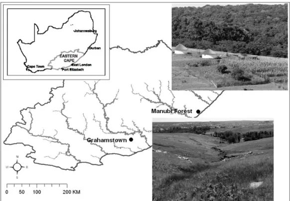
The general objective of this study was to use some short-term detailed evapotranspiration, soil water and weather observations in a forested catchment (Manubi Forest, Figure 1), as well as some simple periodic stream flow observations in a small, relatively steep topography, grassland catchment (Grahamstown, Figures 1 and 2) to assess the structure of a hydrological model that has been used widely within southern Africa for water resources availability assessments (Pitman, 1973; Hughes, 2004). The assessment included an evaluation of the validity of the model algorithms, as well as issues related to establishing appropriate parameter sets and problems of equifinality (Beven, 2006). Specifically, the Manubi Forest data are used to assess the ability of the model to simulate the soil moisture water balance which will be dominated in this catchment by rainfall inputs and evapotranspiration outputs. The focus of the assessment in the Grahamstown catchments is on the model functions that generate stream flow outputs as drainage from the main moisture storage, whether the field observations could help to identify the main runoff generation processes and whether the model is able to realistically simulate their variations over time. Inevitably, the latter also provides some tests of the ability of the model to
simulate the soil moisture water balance, despite the fact that no explicit field observations of soil moisture or evapotranspiration losses have been collected.
It is important to note that the purpose of this study was not to further develop the model, but to assess the model structure and performance using more detailed (in space and time) data than would be available under typical water resources assessment applications of the model.
Any changes that are made to the structure of the model have been made to improve the compatibility of the model outputs with the data used to evaluate them.
STUDY SITES AND FIELD DATA COLLECTION METHODS
Manubi Forest
The Manubi forest (32.451° S; 28.596° E) is a state-owned mixed-species, mixed-age evergreen indigenous forest, located in the coastal region of the Eastern Cape Province of South Africa (Figure 1). It is approximately 760 ha in extent and ranges in elevation from 150 to 230 m.a.s.l. It is classified as a Transkei Coastal Scarp Forest type, within the broader Scarp Forest Group (Mucina and Rutherford, 2006) and it is dominated by Chionanthus peglerae, Strychnos mitis, Drypetes gerrardii, Olea capensis subsp. macrocarpa, Vepris lanceolata and Syzygium gerrardii in the canopy. The sub-canopy is dominated by Englerophytum natalense, Allophylus dregeana, Diospyros natalensis and Tricalysia lanceolata. Trichocladus crinitus and Buxus natalensis form the major component of the sparse to dense shrub understorey (Geldenhuys and Rathogwa, 1995). The Manubi Forest is characterised primarily by very rich doleritic soil, with approximately 30% of the forest underlain by soils derived from Beaufort shales (King, 1940) and the mean annual rainfall is approximately 1070 mm (Schulze and Lynch, 2007).
Weather data (solar radiation, maximum and minimum temperature and relative humidity, wind speed, wind direction and rainfall) were recorded on an hourly basis from 1 Sep. 2010 to 5 Sep. 2011 using an automatic Weather station (Campbell Scientific Inc., Logan, Utah, USA) positioned in an open grassed area at 32.441°S and 28.611°E, at an elevation of 180 m.a.s.l. Volumetric soil water content within the forest was recorded hourly in the top 100 mm of the soil profile from 1 Sep 2010 to 5 Sep 2011, using a CS616 Soil water content probe (Campbell Scientific Inc., Logan, Utah, USA). As all of these measurements are at a single point, the model is also applied as a point water balance model, rather than as a catchment model. The local slope is approximately 1.2o and therefore the influence of lateral flows is assumed to be small.
Total evaporation (ETa) was measured using the Eddy Covariance (EC) technique over three short field campaigns representing spring (3 to 7 Sep. 2010), summer (24 Feb to 2 Mar 2011) and winter (11 to 18 May 2011). Sensors were mounted on a Clark WT8 pneumatic telescopic mast positioned approximately 250m from the northern boundary of the forest and 2.75km from the southern boundary of the forest (32.443°S; 28.609°E) at an elevation of 172 m.a.s.l. Due to fetch limitations associated with the predominantly north/south wind direction, sensors were mounted at 18 m above ground (2.5 m above maximum canopy height). This allowed for a maximum upwind measurement footprint of 250 m. The EC technique is reliant on the shortened energy balance approach (Thom, 1975), which requires estimates of all the components of the energy balance equation (Eq. 1):
= 0
−
−
− G LE H
R
n Equation 1where Rn (W m־²) is the net (incoming minus reflected) solar and thermal irradiance above the canopy surface, G (W m־²) the energy required to heat the soil (soil heat flux), LE (W m־²) the energy required to evaporate water (latent energy flux) and H (W m־²) the energy required to heat the atmosphere above the soil (sensible heat flux). Rn was measured using a net radiometer (Model 240-110 NR-Lite, Kipp & Zonen, Delft, Netherlands). G was measured in the forest floor using soil heat flux plates (model HFT-S, REBS) buried 80 mm below the soil surface, together with soil temperature averaging probes set at 20 mm and 60 mm below the soil surface and time domain reflectometer water content sensors (CS616, Campbell Scientific Inc., Logan, Utah, USA) in the upper 100 mm of the soil. H was measured with a CSAT3 three-dimensional ultrasonic anemometer (CSAT3, Campbell Scientific Inc., Logan, Utah, USA). LE was measured with a LiCor LI-7500 open path infrared gas analyser (IRGA). Measurements conducted at 20Hz and averaged every 30 minutes were stored on a CR5000 data logger (Campbell Scientific Inc., Logan, Utah, USA). The Leaf Area Index (LAI) of the forest was recorded during each field campaign using a LAI2000 plant canopy analyzer (LiCor, Lincoln, Nebraska).
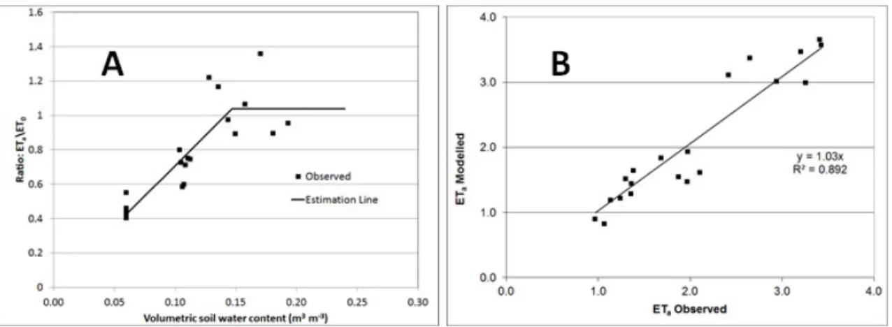
Observed weather, soil moisture and seasonal ETa data were used to estimate daily actual ETa data for the year (Sep 2010 to Oct 2011). The approach followed was to calculate reference ET0 using version 3.1.07 of the software REF-ET (http://www.kimberly.uidaho.edu/ref-et/index.html) and to express daily measured ETa from the EC field campaigns as a fraction of ET0. Reference evapotranspiration, as defined in the software, is the ET that occurs from a "reference" crop such as clipped grass or alfalfa and is consistent with internationally accepted methods (Allen et al., 1998). Measurements taken during each field campaign showed LAI in this evergreen forest to be relatively constant, ranging from 3.5 to 3.6. Seasonal variations in ETa could therefore not be attributed to
changes in leaf area. However, soil water content did vary markedly through the year, and was considered to be the most likely cause of variations in ETa. Consequently, the ratio ETa/ET0 was plotted against volumetric soil water content in the topsoil to derive a two- component relationship between soil water content and the ETa/ET0 ratio (Figure 3A). The two lines were regressed against two groups of points describing each segment of the relation and the regression equations were used to estimate ETa from soil water content and ET0 over the entire year. There are some ratios of ETa/ET0 that exceed 1 and these were attributed to the greater evapotranspiration potential of forests compared to a reference grass cover caused by the higher leaf areas, aerodynamic roughness, rooting depths and soil water availability associated with forests (Bosch and Hewlett, 1982). These higher ratios were noted during the winter months when the available energy was relatively low (i.e. lower ET0) but when the evergreen trees would have access to deeper soil water reserves (i.e.
higher ETa). There are clearly a number of uncertainties associated with this approach (related to the estimates of ET0, the limited depth of the soil moisture data, as well as the EC observations of ETa) but Figure 3B indicates that the estimated daily ETa data are good approximations of the measured ETa values from the three EC field campaigns, the slope estimate (1.03) having a standard error of 0.035.
Grahamstown catchment
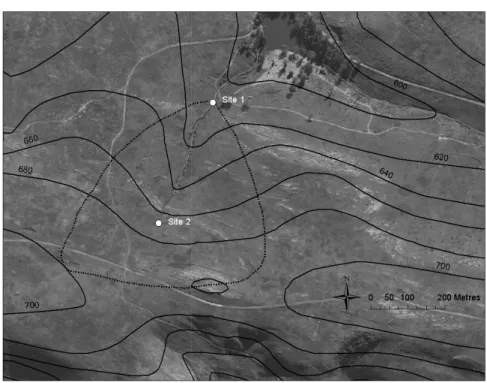
The Grahamstown site (outlet located at 33.326° S; 26.526° E) consists of a first order, steep, grassland catchment underlain by Quartzites of the Witteberg group and has a single incised river channel (Figures 1 and 2). The catchment slopes vary from about 17% in the headwaters to 40% at the point where the channel enters the incised gulley. The majority of the catchment slopes are approximately 18 to 22%, while the channel has a slope of 13%.
Soils vary in depth from very shallow near some rock outcrops, through shallow (< 300mm) on the main slopes and up to 700 mm in the flatter headwater areas. In the valley bottom, surrounding the incised channel, the colluvial deposits can be over 3 m deep and there is clearly visible evidence of preferential subsurface pathways (pipes). These appear to occur at the interface of the sandy loam top soils (with a high organic content) and deeper clay soils of the valley bottom colluvium or hard rock on the slopes. The vegetation cover consists of quite dense grassland that has not experienced burning during the study period.
Daily total rainfall observations were sourced from a site some 1.2 km away, but it should be recognised that rainfall can be quite spatially variable in this hilly terrain. Stream flow measurements at the outlet (catchment area of 0.2 km2) and at a point close to the start of the channel incision (area of 0.03 km2) were started in January 2011 (Figure 2). A simple
measurement system was used based on the time taken to fill a bucket of a known volume (repeated 5 times for each measurement). Some 60 observations are available up to August 2012 with an approximate weekly interval, coupled with several more intense sampling periods immediately after heavy rainfall events. Daily weather station data are available from the Rhodes University campus located approximately 2 km from the site and include
estimates of ET0 as part of the data logger outputs
(http://www.ru.ac.za/static/weather/ARCHIVE/NEWSTATION/RU-Estates; Accessed August 2012). While Figure 2 shows the assumed total catchment boundary, there is some doubt about the exact location in the southern headwater area, partly due to the presence of a gravel road that will inevitably affect drainage directions and partly due to quite complex localised slopes (not evident from the 20m contours shown on Figure 2).
The original reason for investigating this site was to try and identify if there are any differences in the sources of runoff between the small headwater catchment and the lower catchment. It was initially postulated that the downstream catchment would experience more prolonged flow during dry periods and that some of this flow might be derived from interflow within near surface fracture zones below the soil (Hughes, 2010b).
THE HYDROLOGICAL MODEL
The Pitman model is a monthly time-step, semi-distributed (sub-catchment) conceptual, rainfall-runoff model that was developed in 1973 (Pitman, 1973) and has seen a number of modifications since then (Hughes, 2004). A detailed description of the model is available in Hughes et al. (2006). In this study the same (or similar) main water balance algorithms have been implemented in a daily version of the model so that the outputs can be more directly compared to the field data collected at the two sites. In most cases (surface runoff, evapotranspiration from moisture store, groundwater recharge, soil water outflow) exactly the same algorithms that are used in the monthly model can be applied in the daily version.
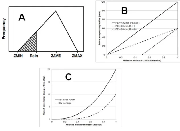
Figure 4A illustrates the approach to surface runoff generation that uses a triangular distribution (parameters ZMIN, ZAVE and ZMAX) to define the frequency of catchment absorption rates. The rainfall rate in any time step can then be used to calculate what proportion of the catchment will exceed the absorption capacities as well as the volume of runoff. Surface runoff is not expected in the Manubi Forest site (low slopes, well vegetated and well drained soils), while only relatively small volumes of surface runoff during intense rainfall are expected for the Grahamstown site. This component of the model is therefore not important for this study.
Figure 4B illustrates the simple linear relationship used to estimate actual evapotranspiration loss from the main (soil) moisture store. As the potential evaporation (PE) rate reduces, the parameter (0<R<1) defines the rate at which actual evapotranspiration declines as the relative moisture content decreases. The potential evaporation input to the model is assumed to be based on Symons pan values and will be different to the reference ET0
derived using the REF-ET software. Equation 2 defines the algorithm for the estimation of actual evapotranspiration (all values in Equations 2 to 4 are in either mm (for storages) or mm per model time unit (month or day) for moisture fluxes).
ETaj = PEj x (Sj/ST) + R X (PEj – PEMAX) * (1 – Sj/ST) Equation 2 Where: ETaj = Actual evapotranspiration in the model time interval j,
PEj = Potential evaporative demand,
PEMAX = Maximum potential evaporative demand, Sj = Current unsaturated zone moisture storage,
ST = Maximum capacity of the unsaturated zone moisture storage, R = Evaporation parameter.
Figure 4C illustrates the non-linear relationships assumed between runoff and groundwater recharge from the moisture store as the relative content of the store changes. These relationships are defined by maximum values when the moisture store is full, power parameters (2.5 for runoff and 4.0 for groundwater in Figure 4C) to define the non-linearity and a minimum moisture store when outflows cease (Equations 3 and 4).
QIj = FT x ((Sj – SLQI) / ST)POW Equation 3
GRj = GW x ((Sj – SLGR) / ST)GPOW Equation 4
Where: QIj = Interflow runoff (from the soil and near surface fracture zones), GRj = Recharge to groundwater,
FT = Maximum interflow runoff,
GW = Maximum groundwater recharge,
POW = Power parameter for the interflow equation, GPOW = Power parameter for the recharge equation,
SLQI & SLGR = Minimum unsaturated zone storages below which QI and GR cease.
In the case of the interception component it was necessary to create a modified algorithm.
This was based on the same principles as used in the monthly model, but using a different
equation. The approach assumes that the product of the vegetation cover fraction and LAI gives the proportion of the surface that can intercept rainfall (COV), while a canopy capacity parameter is used to quantify the maximum canopy storage (CAP). COV * daily rainfall depth is added to the previous days canopy storage (CS), while COV * potential evaporation * CS/CAP is removed. The potential evaporation that is used to estimate soil evapotranspiration is reduced by the amount that is satisfied by evaporation from interception storage.
The monthly version of the model includes groundwater storage and drainage components as well as flow attenuation routing components. The Manubi site is a plot study, while the Grahamstown sites are in elevated topographic positions and the channels are very unlikely to receive groundwater drainage. These model components are therefore not considered applicable to the study sites and were therefore not included in the daily model. In summary, the focus of the assessments of the daily version of the model were on the main unsaturated zone storage water balance components that include rainfall losses to interception and storage losses to evapotranspiration, recharge and runoff.
The model was evaluated for all sites (Manubi and the two Grahamstown sites) using a version that generates 1 000 ensembles with uncertainty ranges for those parameters that are considered to be critical or uncertain. The ensembles are generated using independent random sampling from uniform distributions specified by minimum and maximum likely parameter values. The initial ranges were set to be quite large to ensure that all possible parameter combinations were accounted for. Three objective functions are calculated for the stream flow, soil moisture and actual evapotranspiration (where the equivalent observed data exist) simulated by each ensemble. The objective functions are the Nash Coefficient (Nash and Sutcliffe, 1970) using untransformed data (CE), natural log transformed data (CE(ln)) and inverse transformed data (CE(Inv)). The outputs (all parameter values and objective functions) were ranked using different combinations (dependent on the availability of observed data) of the objective functions and new parameter ranges established to further constrain the parameter space for subsequent model runs. A further output consists of the minimum and maximum simulated values (from all the ensembles) of stream flow, soil moisture and actual evaporation for each time step.
DATA ANALYSIS AND MODEL SIMULATION RESULTS
Manubi Forest data
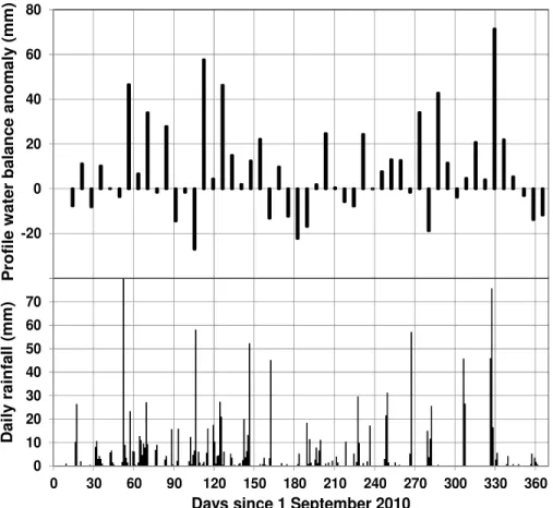
Before any field data can be compared to outputs from the daily version of the Pitman model it is necessary to ensure, as far as possible, that the two data sets are representing the same information. It is also important to assess the field data from the Manubi Forest site from a water balance perspective. The AGIS (2007) landtype data suggest that the soils in this area are silty loams to silty clay loams between 300 and 900 mm deep with a total soil profile moisture storage of between 114 and 342 mm assuming a porosity of 0.38. The field data only measure the soil moisture in the upper 100 mm of soil and it is highly likely that the field moisture content data will under-estimate the profile moisture content in a non-linear manner, more at low, than high measured moisture contents. The field data were checked for a satisfactory water balance by calculating the 7 day anomalies based on the difference between measured soil moisture estimates (SMi and SMi+7, for day i and day i + 7) together with the rainfall and actual evapotranspiration (ETa) over the 7 day periods (Equation 5):
Anomalyi+7 = SMi + ƩRain - ƩETa – SMi+7 Equation 5
Positive anomalies in Equation 5 would be expected due to the possible occurrence of runoff and soil water drainage (lateral and vertical as groundwater recharge) during wet conditions, while negative anomalies represent errors in some part of the water balance estimate because lateral inflows are unlikely given the elevated position of the monitoring site. Figure 5 plots the daily rainfall and the 7 day anomalies for the whole period of data collection and it is clear that there are at least 3 periods (days 90-100, 170-190 and 350-370) of substantial negative anomalies, confirming suspicions that the surface observations are inadequate representations of the real soil profile content. It is worth noting that the 170-190 days period contains the 2nd EC field campaign, when estimates of ETa are expected to be accurate.
The Pitman model was initially applied with existing regional information (Midgley et al., 1994) to define both the annual potential evaporation demand and fixed seasonal distributions. The second approach was to use the daily field estimates of ET0 to define the daily variations in potential evaporation, but with the same annual demand. The regional value for the mean annual potential evaporation (1 250 mm) was increased by up to a factor of 1.2 to allow for possible increased water use by the forest vegetation. The simulated total actual evapotranspiration (equal to interception loss plus soil evapotranspiration in the model) values were compared to the field estimated ETa values, while the field estimated soil moisture values were based on the percentage volume observations from the top 100 mm converted to mm of storage using the same storage capacity (ST) value used in the model and assuming a porosity of 0.38.
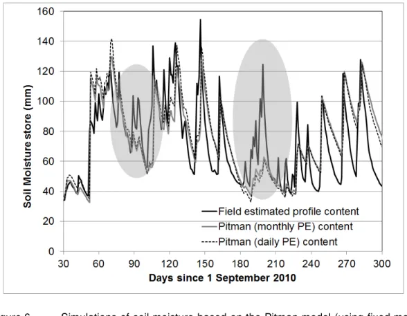
Figure 6 illustrates the results for soil moisture using one of the ensembles that produced some of the highest objective function values for both ETa and soil moisture. However, the objective function values were relatively poor being generally less than 0.5 for soil moisture (regardless of the data transformation). The model results for total actual evapotranspiration showed improvement when the annual potential evaporation demand was distributed with the daily variations in field ET0 data (objective function values up to 0.72) compared to using fixed seasonal distributions (CE and CE(ln) values less than 0.3). Figure 6 illustrates that the main soil moisture simulation problems occur in the periods (highlighted) which have negative water balance anomalies in the field data (Figure 5). Other problems are associated with the much steeper recessions of the field estimated soil moisture values relative to the simulated values. These patterns were evident in all of the initial ensembles to a greater of lesser extent and were also reflected in generally under-simulated ETa values for the same periods highlighted in Figure 6.
These initial results are consistent with the previous conclusion that the field measured soil moisture data are unlikely to represent the full soil profile. In an attempt to overcome this discrepancy between the model outputs and field data, a 2-layer version of the model was established using the same basic modelling structure as the single layer version. The upper layer was defined using a maximum soil water content (STU) of 38 mm (representing 100 mm of soil with a porosity of 0.38). Drainage to the lower layer (DRj) was estimated using the same function as Equation 3, but with new parameters (DFT replacing FT and DPOW replacing POW; Equation 6) and including any rainfall inputs in excess of the maximum storage.
DRj = DFT x (SUj / STU)DPOW Equation 6
Where DRj = Drainage from upper layer to lower layer.
SUj =Current storage in the upper layer.
The net potential evaporation demand (after interception loss) was partitioned between the upper and lower soil layers and the actual evapotranspiration from both layers calculated using Equation 2. The lower soil layer was then simulated in exactly the same way as within the single layer model.
During the first run of the 2-layer model using large parameter uncertainty bounds, a high degree of equifinality was evident in the outputs. The parameter ranges for those ensembles that generate objective function values (soil moisture and ETa) greater than 0.7 were very
similar to those that generated lower CE values. The only clear indication was that the lower annual potential evaporation values generally gave improved results and therefore the scaling factor to allow for increased forest water use was not included in subsequent model runs. In an attempt to reduce the parameter space and therefore the uncertainty in the outputs, some of the parameters were fixed, or had their ranges reduced, based on the following reasoning and assumptions (Table 1):
• Interception was assumed to be close to 20% of rainfall (Dye and Versfeld, 1992;
Everson et al., 2006) and this was achieved with a fixed interception loss parameter of 1.4 mm.
• Infiltration excess surface runoff was assumed not to occur in this forested area and ZMIN was set to greater than 100 mm d-1.
• Groundwater recharge is expected to be approximately 10 to 15% of rainfall, based on previous regional chloride mass balance calculations (DWAF, 2005), and this was achieved with narrow ranges for GW (2 to 3 mm d-1) and GW (2.5 to 3.5).
• Interflow runoff is also expected to be relatively low, associated with the low topographic gradient at the observation site (FT constrained to between 2 and 6 mm d-1, POW to between 3 and 5).
• The upper layer evapotranspiration parameter R was set to 0 on the assumption that evapotranspiration from the upper layer is unlikely to cease even at very low soil moisture levels, while the lower layer R was allowed to vary between 0.2 and 0.6.
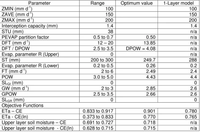
The main focus of the uncertainty assessment (Table 1) was therefore on the maximum lower layer zone storage capacity (ST), the lower layer evapotranspiration parameter (R) and the upper soil layer drainage parameters (DFT and DPOW). It was also noted during the initial run that certain combinations of DFT and DPOW were more behavioural than others.
The model was therefore modified to estimate DFT and DTF/DPOW (rather than DPOW directly) with uncertainty ranges of 12 to 20 mm d-1 and 2.5 to 3.5, respectively. The factor that partitions the evaporation demand between the upper and lower layers was varied between 0.5 and 0.7.
Table 1 includes the range of parameters and objective function values (CE and CE(ln)) for all 1 000 ensembles, as well as the parameter values and results for one of the ensembles that was selected as the best result based on all the objective functions. Figure 7 illustrates the full range of simulated upper layer soil moisture content values compared to the field estimated values and Figure 8 presents the best result for soil moisture. Figure 9 illustrates
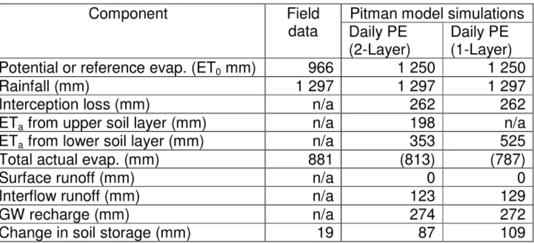
the relationship between the ensemble extremes of simulated ETa compared to the field estimated ETa values, while Figure 10 presents the ETa times series for the best overall ensemble. Table 2 lists the water balance components of the best ensemble output and compares the results with the observed data where available. Figure 10 as well as the very high objective function values indicate that the ETa simulations have been improved a great deal and the under-simulation of actual evapotranspiration by the original single layer model during certain periods has been corrected.
The final model run used the original single layer model with parameters inferred from the 2- layer model best results. Table 1 includes the parameter values and objective function results (for ETa only), while Table 2 includes all the water balance components. The ETa
simulations are somewhat better than those obtained from the original exploratory runs of the single layer model, largely because the 2-layer model results pointed toward different parameter combinations, notably much higher soil moisture storage. The simulations of the total soil moisture content for the final single run of the 1-layer model and the best result for the uncertainty 2-layer model are also very close. The conclusion is that the two models are simulating the overall water balance in the same way, but that the inclusion of a second layer improved our ability to determine appropriate parameter values and assess the model results relative to the observed data. One notable feature of the soil moisture simulations (Figure 7) is the fact that high observed soil moisture levels tend to follow the upper bound of the uncertainty ensemble outputs, while lower observed values tend toward the lower simulation bounds. The implication, which is confirmed by Figure 8 that shows the best simulation result, is that no single set of parameters is apparently able to simulate the full range of observed soil moisture values.
Grahamstown catchment data
Some initial simulations using the original single layer model were performed with an annual potential evaporation value (1552 mm) and fixed monthly distributions obtained from Midgley et al. (1994), as well as with daily ET0 data calculated from the weather station data to distribute the same annual value. The main differences in the two seasonal distributions of evaporation demand were during the winter months, with the ET0 based estimates suggesting a much more evenly distributed demand than the regional values from Midgley et al. (1994). The daily data produced (not unexpectedly) improved simulations and therefore all the later simulations were based on using the daily ET0 data.
The model was evaluated for the Grahamstown sites (upper and total catchment) based on two sequences of running the model to generate 1 000 ensembles. The initial ranges were set to be quite large to ensure that all possible parameter combinations were accounted for.
The outputs (all parameter values and objective functions) were ranked using the CE(ln) and CE values and the new parameter ranges for the second model run based on those ensembles that generated CE and CE(ln) values of greater than 0.7. Many of the CE(Inv) values were very low and this objective function was not used to assess the initial parameter ranges. There was a lower degree of equifinality in the Grahamstown parameter sets than was evident for the Manubi Forest site and it was possible to constrain the behavioural parameter space after the first run. The following additional guidelines were used to further constrain the parameter ranges of the second sequence to ensure that the results were not biased by unrealistic parameter sets:
• ZMIN and ZMAX values were set to generate surface runoff only during rainfalls of greater than 50 mm d-1 and have very little influence on the simulations.
• Maximum interception storage was set to 1.0 mm, which is considered to be consistent with the dense and relatively tall grass cover.
• GW, GPOW and SLGR ranges were established to ensure that the mean recharge lay within expected values (DWAF, 2005) of approximately 4% of rainfall.
• ST values were constrained to be within values expected from the knowledge of soil depths and texture (150 to 300 mm).
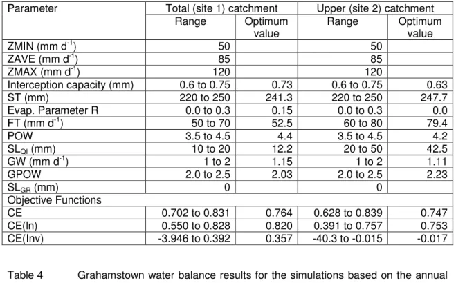
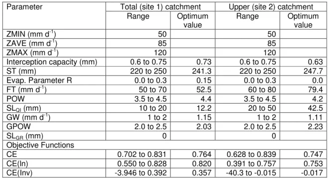
Table 3 summarises the final parameter ranges, the best parameter set (based on combinations of all three objective functions) and also provides the range of objective functions generated by the ensembles. It should be noted that although the objective was to limit the parameter space to achieve CE and CE(ln) values of greater than 0.7, there inevitably remain some parameter combinations that produce lower objective function values during the second run. Figures 11 and 12 illustrate the results compared with the observed daily flow depths and include the upper and lower limits of all the ensembles, as well as the ensemble that was identified as having the best combination of objective function values, with a bias towards the CE(ln) values.
The first notable result is that the observed data tend to follow the upper simulation bounds during wet periods (days 150 to 350), but are generally closer to (or below for site 1) the lower simulation bounds during drier conditions (from day 400 onwards). A conclusion similar to that reached for the soil moisture simulations at the Manubi Forest site. This suggests that the combination of the model structure and input data used are not able to
successfully simulate the full range of observed flows with a single parameter set. This is further illustrated in Figure 13 which plots the CE(ln) values against the CE values. The former will reflect the model performance at low to moderate flows, while the latter will be dominated by the performance at higher flows. Figure 13 illustrates that achieving optimum results for both objective functions is not possible. It is also important to note that the uncertainty bounds are greater during generally dry periods, largely a reflection of the variations in parameters R, POW and SLQI. These results suggest that there are deficiencies in the model structure or in some of the input data when applied at this small spatial scale and/or at the time scale of 1 day. There are several possibilities that can be suggested:
• The model is not simulating enough evapotranspiration during the somewhat drier periods before day 150 and after day 450 when parameter sets are used that successfully simulate the wetter period. This could be related to inadequacies in the input ET0 data, but could also be associated with the relatively simple storage – evapotranspiration loss function used in the model (Figure 4B).
• The non-linearity in the soil moisture storage – runoff function (Figure 4C) is not representing the real non-linearity in runoff response. While this cannot be totally negated, it seems to be less likely than other possibilities as the simulated soil moisture storage conditions during days 500 to 600 are similar to those during parts of the period during days 250 to 350 (Figures 11 and 12) when the observed data remain close to the upper bound simulations.
• A further possibility is that the rainfall data used are not sufficiently representative of the site, despite being observed in the near vicinity. The steep topography of this area, and the expectation of quite high localised variability, make this a very real possibility, but it is impossible to assess without further data.
The apparently inadequate moisture losses during the drier second winter period could be related to the north-facing aspect of the whole catchment and an under-estimate of evaporation demand. The effect is not evident in the winter of the first year (days 160 to 220) as this was a generally wetter period. Scott Munro and Huang (1997) report on the differences in evaporative loss between north and south facing slopes in a Chinese catchment close to the Tropic of Cancer. There results suggest that north facing slopes have approximately 40% of the evaporative losses observed on south facing slopes during winter, with no differences in summer. The effects for the Grahamstown catchment could be even greater (but reversed for the southern hemisphere), given its higher latitude. To test this possible effect, the weather station ET0 estimates were scaled by different amounts (1.2 to 1.4 times higher in mid-winter, no scaling in mid-summer). The simulation results for the
period between 500 and 600 days certainly improved, but the overall ensemble results and objective function values remained very similar to those presented in Figures 11 and 12 and Table 3. The benefits of this change to the input data could therefore not be confirmed.
The uncertainty range for the maximum soil store (Table 4) is somewhat higher than suggested by a field survey of soil depths but it is very difficult to estimate a representative value given the large variations between the slopes and the incised channel area. The field estimates also do not account for the influence of weathered material at the base of the soil profile. The relatively high maximum soil moisture runoff parameter values (50 to 80 mm d-1) are considered to be realistic and consistent with field observations of rapid sub-surface pipe flow during wet conditions throughout the length of the incised channel banks. This could also account for rapid reductions in simulated runoff as the soil moisture content reduces (POW values of 3.5 to 4.5) and some pipes dry out. The relatively high value for the soil moisture content at which interflow ceases (SLQI in Table 4) at the upper site could be related to sub-surface drainage flowing beneath the bed of the shallow channel during dry conditions.
DISCUSSION AND CONCLUSIONS
One of the first observations is that data collected in the field do not always measure the same processes that are simulated by a model. In the Manubi Forest study, the soil water content data measured for the top 100 mm is not consistent with the original model set-up that simulates the water balance of the total soil profile. This makes comparisons difficult and it is not surprising that the initial Pitman model results indicate a poor fit to the field data during the same periods as the negative anomalies. Consequently, if soil moisture data are to be collected for model assessment purposes then the data should cover the full soil profile. It was concluded that the observed water balance anomalies for the upper 100 mm of soil are associated with evapotranspiration demands being met from dynamic interactions of the two soil layers. Incorporating a second soil layer into the model allowed more direct comparisons to be made between the field and simulated soil moisture values and generated much improved simulations. However, it is not suggested that routine applications of the Pitman model should include a 2-layer soil moisture storage algorithm, and it was only included in this study to facilitate the comparison between the model results and the field data. The original, single layer, version of the model was able to simulate (after revisiting likely parameter bounds) the same patterns of water balance variation as the 2-layer model.
The Manubi Forest study indicated that replacing fixed seasonal distributions with field ET0
estimates generates much improved simulations of actual evapotranspiration, but makes much less difference to simulations of soil moisture or to the overall water balance components. A similar conclusion was reached about the use of daily ET0 estimates from local weather station data for the Grahamstown sites. This effect is likely to be far more apparent in the application of the daily version of the model than the more typically used monthly version. It is also important to note that for all of the simulations the absolute values of estimated ET0 are too low to be used directly in the Pitman model which was originally designed to use evaporation pan data as input. It is not possible to simply modify the other parameter values to get acceptable simulations if the ET0 data are used directly. The implication is that if ET0 data are to be used with the Pitman model there would have to be some structural changes to the simple linear relationship (Figure 4B) between evaporative demand, soil moisture storage and actual evapotranspiration losses. Investigating possible changes to the model evapotranspiration algorithm was beyond the scope of this study, but is recommended for the future given the number of global data sets that make use of ET0 for evaporative demand estimates, including the MODIS16 (Mu et al., 2011) products. There is little doubt that the standard monthly distributions of evaporation demand that have been published (Midgley et al., 1994) are not always appropriate, but it is possible that this issue is related to catchment scale and that the published values are appropriate for the much larger catchments in which they are normally used. There may also be other conditions under which the Midgley et al. (1994) distributions are acceptable, but this study did not pursue this issue any further.
Both sites confirmed the high degree of equifinality in the structure and parameter sets of the Pitman model, a consequence of the relatively large parameter space for a conceptual type model. The Manubi Forest site illustrates that using two sets of field observation data (soil moisture and ETa) does not necessarily help to resolve the issues of equifinality and lack of parameter identifiability, which were made worse because of the additional parameters associated with the extra soil layer. The problem was less evident for the Grahamstown sites where the single layer model was used. It is also possible that observed stream flow data contain more parameter identification signals than soil moisture and ETa data. Additional information from various sources was used at both sites to further constrain some of the parameter values, particularly those related to the interception and groundwater recharge components of the model. None of these information sources are site specific but can nevertheless be considered useful to constrain the uncertainty in behavioural parameter sets. This is similar to the approach using regional signatures of hydrological behaviour adopted by Yadav et al. (2007) and others.
One of the objectives of the Grahamstown study was to identify if there are differences in low flow response between the very small headwater catchment and the total catchment as well as between wet and dry periods. This was part of the objective to try and use models to improve the understanding of the runoff generation processes (Beven, 2012). It was initially considered possible that during dry conditions the flows in the lower part of the catchment might be derived from near surface fractured rock seepage (Hughes, 2010b). However, the model simulations do not support this concept and neither do isotope samples collected for both sites during a wet and dry period. Both sites show similar degrees of enrichment, with the dry season samples showing greater evaporative enrichment, consistent with drainage from the soil profile.
The simulations for both studies appear to be generally behavioural with parameter sets and water balance components that are consistent with what is known. This suggests that the main water balance algorithms of the Pitman model are generally acceptable even for small catchments, given appropriate input data. However, both studies have identified that there are either some potential structural weaknesses or possible input data problems and illustrate the importance of covering a range of wet and dry conditions (Siebert and Beven, 2009) in all seasons of the year. Figures 7, 8, 11 and 12 suggest that a single set of parameters do not provide equally good simulations for both wet and dry conditions, particularly during winter months. Without more detailed information, it has not been possible to conclusively ascribe these effects to any specific component of the model, a weakness in any specific model algorithm or a lack of representative climate inputs. It is likely to be a combination of several factors and uncertainties in the input climate data (rainfall and evaporative demand) would need to be resolved before any attempts could be made to realistically modify the structure of the model. It is also difficult to conclude whether these effects have identified a possible weakness in the overall model concepts, or whether they might be specific to the daily version that has been applied in this study. The total period of the Grahamstown study represents a particularly wet period, notably so for the two winter seasons covered. It is possible that monitoring through an extended dry winter period might provide additional information that could clarify some of the remaining uncertainties. If the study were to be extended, it would be necessary to improve the monitoring of the local rainfall patterns and certainly worthwhile trying to obtain some site specific ET0 estimates.
The overall conclusion of the study is that even the simple type of field data collected for the Grahamstown sites has been valuable in assessing the structure of a daily implementation of the Pitman model and for constraining the behavioural parameter space. It is concluded that
the structure of the model is generally appropriate, even for simulating the hydrological response of much smaller catchments than those for which it was designed. However, there remain some unresolved uncertainties about the low flow processes in the Grahamstown catchment and the way in which these are simulated by the model. The more detailed field data collected for the Manubi Forest site has allowed the study to demonstrate that the model is able to simulate more than just stream flow responses with acceptable degrees of accuracy. It is also evident from the study that a daily time-step implementation of the Pitman model, normally only applied at monthly time steps, is viable and should be pursued as a future development. However, it is also recommended that applications of a daily version of the model should be accompanied by more detailed evaporation demand data than is typically used with the monthly model. This may involve estimates based on nearby weather station data or using time series from MODIS data for example.
Finally, it is appropriate to emphasise that the purpose of this study had somewhat different objectives to many other studies that have assessed the use of field observations to improve the structure or parameters of hydrological models (Fenicia et al., 2008; Clark et al., 2011;
McMillan et al., 2011). For example, Clark et al. (2011) and McMillan et al., (2011) recommended the development of unique model structures for individual catchments and that available data should be used to develop uniquely appropriate model structures. This study has applied the Pitman model which is widely used in water resources assessments and water resources allocation decision-making within southern Africa, a generally data scarce region. It would therefore not be practical to suggest that this model is replaced by unique models for every catchment or part of the region. While the conclusions of Clark et al.
(2011) and McMillan et al. (2011) are applicable to the development of the science of hydrology, this study has focussed on using hydrological science to try and support the practical application of a specific model. The authors therefore contend that the paper makes a contribution to the debate about ‘getting the right answers for the right reasons’ (Kirchner, 2006) and spans the hydrological science and water resources engineering domains of catchment hydrological modelling.
ACKNOWLEDGEMENTS
The data for the Manubi forest area were obtained from a research project (K5/1876,
"Water-use and economic value of the biomass of indigenous trees under natural and plantation conditions"), solicited, managed and funded by the Water Research Commission (WRC, 2010) with co-funding from the Working for Water Programme of the Department of Environmental Affairs, and undertaken by the CSIR. The South African Dept. of Agriculture,
Forestry and Fisheries (DAFF) are thanked for granting permission to conduct research within the Manubi State Forest. Mr. Vivek Naiken (CSIR) and Mr. Thembelani Nokwali (DAFF) provided assistance with installation and maintenance of equipment at the site. Ms Tanner participated in the study as part of her PhD programme which is jointly funded by the Regional Initiative in Science Education (RISE) programme of the Carnegie Foundation of New York, the Water Research Commission through project K5/2056 and a DAAD/National Research Foundation studentship (UID: 74109). The authors are very grateful for the extremely pertinent comments provided by the anonymous reviewers and the associate editor of the journal that contributed many improvements to the paper during the review process.
REFERENCES
AGIS. 2007. Agricultural Geo-Referenced Information System, accessed from http://www.agis.agric.za (Accessed June 2012).
Allen, RG, Pereira, LS, Raes, D and Smith, M. 1998. Crop evapotranspiration: Guidelines for computing crop water requirements. FAO Irrigation and Drainage Paper 56. pp 300.
Banks, EW, Simmons, CT, Love, AJ and Shand, P. 2011. Assessing spatial and temporal connectivity between surface water and groundwater in a regional catchment:
Implications for regional scale water quantity and quantity. Journal of Hydrology 404, 30-49.
Beven, K. 2006. A manifesto for the equifinality thesis. Journal of Hydrology 320, 18-36.
Beven, K. 2012. Causal models as multiple working hypotheses about environmental processes. C.R.Geoscience 344, 77-88.
Bosch, JM and Hewlett, JD. 1982. A review of catchment experiments to determine the effect of vegetation changes on water yield and evapotranspiration. Journal of Hydrology 55, 3-23.
Clark, MP, McMillan, HK, Collins, DBG, Kavetsi, D and Woods, RA. 2011. Hydrological field data from a modeller’s perspective: Part 2. Process–based evaluation of model hypotheses. Hydrological Processes 25(4), 523-543.
Clulow, AD, Everson, CS and Gush, MB. 2011. The long-term impact of Acacia mearnsii trees on evaporation, streamflow, and ground water resources. Water Research Commission Report No.TT505/11, WRC, Pretoria, South Africa.
DWAF. 2005. Groundwater Resource Assessment II. Department of Water Affairs and Forestry, Pretoria, South Africa.
Dye, PJ and Versfeld, DB. 1992. Rainfall interception by a ten year old Pinus patula plantation. Unpublished contract report to the Dept. of Water Affairs and Forestry,
FOR-DEA 424. Division of Forest Science and Technology, CSIR, Sabie, South Africa.
Everson, C, Gush, M, Moodley, M, Jarmain, C, Govender, M and Dye, P. 2006. Can effective management of riparian zone vegetation significantly reduce the cost of catchment management and enable greater productivity of land resources. Water Research Commission Report No. K5/1284, Pretoria, South Africa.
Everson, CS, Dye, PJ, Gush, MB and Everson, TM. 2011. Water-use of grasslands, agro- forestry systems and indigenous forests. Water SA 37 (5), 781-788.
Fenicia, F, McDonnell, J and Savenije, HHG. 2008. Learning from model improvement: On the contribution of complementary data to process understanding. Water Resources Research 44(6), W06419, doi: 10.1029/2007WR006386.
Geldenhuys, CJ and Rathogwa, NR 1995. Growth and mortality patterns over stands and species in the Manubi forest increment study site: report on 1995 measurements.
Report FOR-DEA 943, Division of Water, Environment and Forestry Technology, CSIR, Pretoria.
Gupta HV, Wagener T and Liu Y. 2008. Reconciling theory with observations: elements of a diagnostic approach to model evaluation. Hydrological Processes 22, 3802-3813.
Gupta, HV, Clark, MP, Vrugt, JA, Ambrovitz, G and Ye, M. 2012. Towards a comprehensive assessment of model structural adequacy. Water Resources Research 48, W08301, doi: 10.1029/2011WR011044.
Hewlett, JD, Lull, HW and Reinhart, KG. 1969. In defence of experimental watersheds.
Water Resources Research 5(1), 306-316.
Hughes, DA. 1994. Soil moisture and runoff simulations using four catchment rainfall-runoff models. Journal of Hydrology 158, 381-404.
Hughes, DA. 2004. Incorporating ground water recharge and discharge functions into an existing monthly rainfall-runoff model. Hydrological Sciences Journal 49(2), 297-311.
Hughes, DA. 2010a. Hydrological models: mathematics or science? Hydrological Processes 24, 2199-2201.
Hughes, DA. 2010b. Unsaturated zone flow contributions to stream flow: evidence for the process in South Africa and its importance. Hydrological Processes 24, 767-774.
Hughes, DA, Andersson, L, Wilk, J and Savenije, HHG. 2006. Regional calibration of the Pitman model for the Okavango River. Journal of Hydrology 331, 30–42.
Khu, S-T, Madsen, H and di Pierro, F. 2008. Incorporating multiple observations for distributed hydrologic model calibration: An approach using a multi-objective evolutionary algorithm and clustering. Advances in Water Research 31(10), 1387- 1398.
King, NL. 1940. The Manubi forest. Journal of the South African Forestry Association 4, 24- 29.
Kirchner, JW. 2006. Getting the right answers for the right reasons: Linking measurements, analyses and models to advance the science of hydrology. Water Resources Research 42, W03S04, doi:10.1029/2005WR004362.
McMillan, HK, Clark, MP, Bowden, WB, Duncan, M and Woods, RA. 2011. Hydrological field data from a modeller’s perspective: Part 1. Diagnostic tests for model structure.
Hydrological Processes 25(4), 511-522.
Midgley, DC, Pitman, WV and Middleton, BJ. 1994 Surface water resources of South Africa 1990, Volumes I to IV, WRC Report No. 298/1.1/94 to 298/6.2/94. Water Research Commission, Pretoria, South Africa.
Mu, Q, Zhao, M and Running, SW. 2011 Improvements to a MODIS Global Terrestrial Evapotranspiration Algorithm. Remote Sensing of Environment 115, 1781-1800.
Mucina, L and Rutherford, MC. (eds.) 2006. The vegetation of South Africa, Lesotho and Swaziland. Strelitzia 19. South African National Biodiversity Institute, Pretoria.
Nash, JE and Sutcliffe, JV. 1970 River flow forecasting through conceptual models. Part I – a discussion of principles. Journal of Hydrology 10, 282-290.
Scott Munro, D and Huang, LJ. 1997 Rainfall, evaporation and runoff responses to hillslope aspect in the Shenchong Basin. Catena 29, 131-144.
Pitman, WV. 1973. A mathematical model for generating monthly river flows from meteorological data in South Africa. Hydrological Research Unit, Univ. of the Witwatersrand, Report No. 2/73, Johannesburg, South Africa.
Schulze, RE and Lynch, SD. 2007. Annual Precipitation. In: Schulze, R.E. (Ed). 2007. South African Atlas of Climatology and Agrohydrology. Water Research Commission, Pretoria, RSA, WRC Report 1489/1/06, Section 6.2.
Scott, DF and Lesch, W. 1997. Streamflow responses to afforestation with Eucalyptus grandis and Pinus patula and to felling in the Mokobulaan experimental catchments South Africa. Journal of Hydrology 199, 360-377.
Seibert J, and McDonnell JJ. 2002. On the dialog between experimentalist and modeler in catchment hydrology: Use of soft data for multicriteria model calibration, Water Resources Research 38(11), 1241, doi:10.1029/2001WR000978.
Seibert J and Beven KJ. 2009. Gauging the ungauged basin: how many discharge measurements are needed? Hydrology and Earth System Sciences 13(6), 883-892.
Thom, AS. 1975. Momentum, mass and heat exchange of plant communities. In: J.L.
Monteith (Ed.), Vegetation and the atmosphere, Vol. 1, Academic Press, London.
Uhlenbrook, S and Sieber, A. 2005. On the value of experimental data to reduce the prediction uncertainty of a process-oriented catchment model. Environmental Modelling and Software 20(1), 19-32.
Uhlenbrook, S, Didszun, J and Wenninger, J. 2008. Source areas and mixing of runoff components at the hillslope scale—a multi-technical approach. Hydrological Sciences Journal 53(4), 741-753.
Water Research Commission. 2010. Abridged Knowledge Review 2009/10 - Growing Knowledge for South Africa’s Water Future. WRC, Pretoria. pp. 59-60.
Wagener, T and Wheater, HS. 2006. Parameter estimation and regionalization for continuous rainfall-runoff models including uncertainty. Journal of Hydrology 320, 132-154.
Wenninger, J, Uhlenbrook, S, Lorentz, S, and Liebundgut, C. 2008. Identification of runoff generation processes using combined hydrometric, tracer and geophysical methods in a headwater catchment in South Africa. Hydrological Sciences Journal 53(1), 65- 80.
Wooldridge, SA, Kalma, JD and Walker, JP. 2003. Importance of soil moisture measurements for inferring parameters in hydrologic models of low-yielding ephemeral catchments. Environmental Modelling and Software 18(1), 35-48.
Yadav, M, Wagener, T, Gupta, HV. 2007. Regionalisation of constraints on expected watershed response behaviour. Advances in Water Res. 30, 1756-1774.
Zhu, TX, Cai, QG and Zeng, BQ. 1997. Runoff generation on a semi-arid agricultural catchment: field and experimental studies. Journal of Hydrology 196, 99-118.
Table 1 Pitman 2-layer model parameter values and objective function results for the Manubi site simulations (see Figures 3 and 4 and Equations 2 to 4 for explanations of the parameter values).
Parameter Range Optimum value 1-Layer model
ZMIN (mm d-1) 100 100
ZAVE (mm d-1) 150 150
ZMAX (mm d-1) 200 200
Interception capacity (mm) 1.4 1.4
STU (mm) 38 n/a
PEVAP partition factor 0.5 to 0.7 0.50 n/a
DFT (mm d-1) 12 – 20 13.85 n/a
DFT / DPOW 2.5 to 3.5 DPOW = 4.08 n/a
Evap. parameter R (Upper) 0 n/a
ST (mm) 200 to 300 249.7 288
Evap. parameter R (Lower) 0.2 to 0.5 0.26 0.2
FT (mm d-1) 2 to 6 2.49 2.4
POW 3.0 to 5.0 4.43 4.4
SLQI (mm) 0 0
GW (mm d-1) 2 to 3 2.85 2.6
GPOW 2.5 to 3.5 2.66 2.6
SLGR (mm) 0 0
Objective Functions
ETa – CE 0.833 to 0.917 0.901 0.780
ETa - CE(ln) 0.373 to 0.833 0.770 0.765
Upper layer soil moisture – CE 0.691 to 0.727 0.718 n/a
Upper layer soil moisture - CE(ln) 0.628 to 0.715 0.715 n/a
Table 2 Manubi Forest water balance results (all values rounded to nearest mm)
Component Field
data
Pitman model simulations Daily PE
(2-Layer)
Daily PE (1-Layer) Potential or reference evap. (ET0 mm) 966 1 250 1 250
Rainfall (mm) 1 297 1 297 1 297
Interception loss (mm) n/a 262 262
ETa from upper soil layer (mm) n/a 198 n/a
ETa from lower soil layer (mm) n/a 353 525
Total actual evap. (mm) 881 (813) (787)
Surface runoff (mm) n/a 0 0
Interflow runoff (mm) n/a 123 129
GW recharge (mm) n/a 274 272
Change in soil storage (mm) 19 87 109
Table 3 Pitman model parameter values and objective function results for the Grahamstown site simulations.
Parameter Total (site 1) catchment Upper (site 2) catchment
Range Optimum
value
Range Optimum
value
ZMIN (mm d-1) 50 50
ZAVE (mm d-1) 85 85
ZMAX (mm d-1) 120 120
Interception capacity (mm) 0.6 to 0.75 0.73 0.6 to 0.75 0.63
ST (mm) 220 to 250 241.3 220 to 250 247.7
Evap. Parameter R 0.0 to 0.3 0.15 0.0 to 0.3 0.0
FT (mm d-1) 50 to 70 52.5 60 to 80 79.4
POW 3.5 to 4.5 4.4 3.5 to 4.5 4.2
SLQI (mm) 10 to 20 12.2 20 to 50 42.5
GW (mm d-1) 1 to 2 1.15 1 to 2 1.11
GPOW 2.0 to 2.5 2.03 2.0 to 2.5 2.23
SLGR (mm) 0 0
Objective Functions
CE 0.702 to 0.831 0.764 0.628 to 0.839 0.747
CE(ln) 0.550 to 0.828 0.820 0.391 to 0.757 0.753
CE(Inv) -3.946 to 0.392 0.357 -40.3 to -0.015 -0.017
Table 4 Grahamstown water balance results for the simulations based on the annual potential evaporation distributed using daily ET0 estimates and the optimum parameter set (all values are annualised and rounded to nearest mm).
Component Pitman model simulations
Total (site 1) catchment
Upper (site 2) catchment Potential or reference evap. (ET0 mm) 1 552 1 552
Rainfall (mm) 970 970
Interception loss (mm) 133 116
Soil evapotranspiration (mm) 424 506
Total actual evap. (mm) (557) (622)
Surface runoff (mm) 7 7
Interflow runoff (mm) 329 279
GW recharge (mm) 61 51
Change in soil storage (mm) 16 11