Finally, I have a website with the sea ice data and all the code in the book. Ctrl + R (Command Return with Mac) will send the current line to the keyboard editor.
Importing Data into R
In our first example, we define the function f to bex2sin(x) and evaluate it to 3 with f(3). Note that in the second example we define the variable p inside the parentheses of the function, which makes defining the function easier.
A Piecewise-Defined Function
This sets up a graph frame so we can then add the two parts of the piecewise function. An important element of curve is that it graphs only the function in the given x range, regardless of the range of x in the existing graph.
A Step Function
Polar Coordinates
Before creating a graph with polars, we set the lower, left, upper and right edges to 1, 1, 2 and 1 line, respectively. A black frame with bxcol is placed around the graph, which can also be set to FALSE.
Parametric Equations
Inside expression we must use * to juxtapose objects, quotes around text, and double tildas with a space between them to create space between the formulas and the text. The global arguments such as grcol, bxcol and main are omitted, but we color the graph purple and use a dotted line type by setting lty=2.
Geometric Definition of a Parabola
We define the function g as a function of x that will return the value of y that is equidistant between the point (0,1) and the x-axis. The function uniroot.all will return all the roots of the function in the given range from 0 to y.max.
Functions that Return a Function
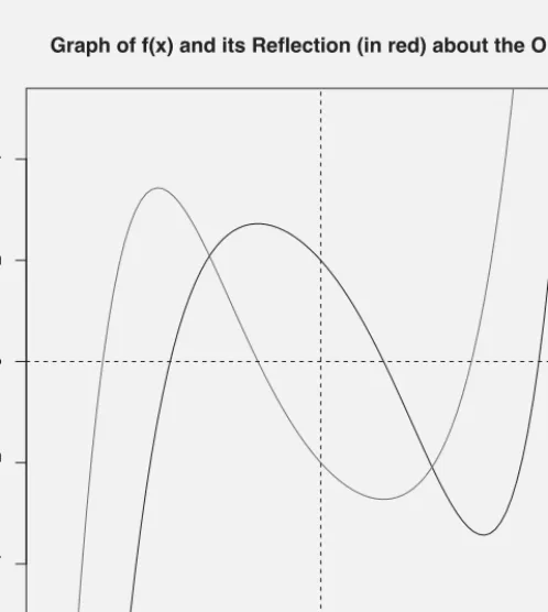
2 to 2, set the y-axis to −5 to 5, label the side axis with the function's expression and add a title with main. We add the graph of its reflection over the origin by drawing Reflect.origin(f)(x)from −2 to 2 and coloring it red.
Pythagorean Triples and a Checkerboard Plot
Note that the function as written assumes that the first input is the smaller of the two return values of asEuclid1(3,2). Arguments can be set to NULL, in which case the lines are at the current graph ticks.
Exercises
The text is justified with the command adj=c(1,1) to the right/above the point (p[2],p[4]) and darkened. The anxcoordinate of p[2]+0.15 places the text outside the graph since p[2] is the rightmost value of the graph.
Graphing Functions
On the other hand, we use the default ticks on the y-axis and NULL places the grid lines along the default ticks. The next two options, cex.axis=1.5 and font=2, scale the labels to 1.5 the default size and make them bold.
Scatter Plots
The first two elements set the coordinates of the text, which were selected by trial and error. Again, cex is used to scale the font size to be 75% of the default size.
Dot, Pie, and Bar Charts
The same can be done for the male data, with the only difference in the pie chart being that the months are labeled one through twelve. If we were to do this in one step with Flabels=paste(FMonth, Fperct, “%”), the vector would have spaces between the percentage values for each month and the % sign.
Boxplot with a Stripchart
The reading from the inside of the loop, when i=1 Month[1] is "Jan", which is the first element of the Month vector. Technically, the function which creates a vector with the location of "Jan" in the FBM and in this case gives
Histogram
To superimpose the normal density, we first calculate the mean and standard deviation of the data and set these values to m and s, respectively. When the add=TRUE argument is included, the feature is added to the current graph.
Exercises
The PolynomF package is designed to do almost anything we want to do with a polynomial. Using the tools of the PolynomF package, we explore the roots of degree-three polynomials, create Pascal's triangle and a Taylor polynomial, and test two Legendre polynomial identities.
Basic Polynomial Operations
We highlight this package by demonstrating basic polynomial operations, arithmetic with polynomials, and working with a list of polynomials. The plot function recognizes polynomial objects and will choose a window containing the maximum and minimum points of the polynomial, as shown in plot(p6).
The LCM and GCD of Polynomials
In this case, the probability of non-constant GCD is a problem of choosing the same integer in each of rand.int.5, rand.int.7, and rand.int.10. An interesting question, left as an exercise, asks what is the chance of getting a non-constant GCD if the polynomials are created with random coefficients instead of roots.
Illustrating Roots of a Degree-Three Polynomial
The second ends the for loop for j, while the third ends the for loop for i. The entries of each are sequence dependent, meaning that the first entries will create the first line of the legend and the same for the second and third.
Creating Pascal’s Triangle with Polynomial Coeffi- cientscients
Our inner for loop varies j from 0 to i and will be used to select the coefficients from the polynomial p. Outside of the if then statement, we place the value on the graph using the text function.
Calculus with Polynomials
For example, poly.info$zeros returns the roots of P(x), while Re(poly.info . $zeros) returns the real part of the roots. Similarly, we can use Im(poly.info$zeros[3]) if we only want the imaginary part of the third root.
Taylor Polynomial of Sin(x)
The first coefficient is sin(0) and so we concatenate sin(0) and the vector coefficient to get Taylor.poly.sin. We set the range for the y-axis with ylim, set the line width to 0 with lwd, and label their axis with ylab.
Legendre Polynomials
Note that if we use P[[5]], the list will only show polynomials by removing the list of polynomials. Now we check the identity Pn′(1) = n(n+ 1)/2, although this time we return both sides of the identity in the question.
Exercises
In other words, the operations on these sequences are applied to each value of the sequence. The basic arithmetic operations used for a sequence are applied to each value, such as cubing and adding 5 in our example.
Sequences and Series
If we later decide to use different lower and upper values for our sequence, this is the only part of the code that will need to be changed. We see from the graph that the behavior of the two series of partial sums looks very different.
The Derivative as a Limit
We needed extra space on the left since our caption is a fraction that takes up extra lines. This graph suggests that the limit is 3, which we know is the derivative of x3at x= 1, but the convergence is not linear.
Recursive Sequences
The next part sets the ith sequence value to the sum of the previous two, i-1 and i-2. Our second example cheats a bit by simply putting our sequence in a 20 by 1 matrix and taking advantage of the extra result.
Exercises
Exercises 101 and compare it to the Fibonacci sequence by drawing the difference between the two sequences. Which graph, from 0 to 1000 or 900 to 1000, is more useful in understanding the behavior of the two sequences of partial sums.
Symbolic Differentiation
The output is not always nice, especially if the derivative gets complicated with a chain rule. We were sloppy here by not specifying that we were requesting the derivative with respect to tox.
Finding Maximum, Minimum, and Inflection Points
Graphing a Function and Its Derivative
The first two arguments of text are the coordinates where text should be placed. The third argument of text is the text to add to the graph, which is defined by one expression to get f′(x).
Graphing a Function with Tangent Lines
The colors of each row will be taken in order from the color vector, but since the color elements are from 1 to 5, we must use i+ 3. In this example, we defined the tangent line as f.tl=function(x ,a ){fp(a)*. x-a)+f(a)}and it works, but only for the specific functionf.
Shading the Normal Density Curve Outside the In- flection Pointsflection Points
Shading the normal density curve outside the inflection points 115 with dots you can enter a list of x values and the corresponding values can be evaluated by a function. Our final goal is to shade the tail of the density curve starting at the inflection points.
Exercises
In our last line, f(mid) is the list of values created by evaluating each element of mid byf. Thenf(mid)*dx multiplies each element of f(mid) by dx, creating a list of the areas of each box.
Riemann Boxes
For mid.box.y, two of the y values are 0 and the other two are obtained by evaluating the function mid[i]. In this case, we aligned the text to the left and top of the location.
Numerical Integration
Computing an iterated integral with R requires the use of sapply, so we'll start with two examples that illustrate sapply. To complete the calculation, we simply wrap an integral around the function of y, created from the sapply example, which is the following example.
Area Between Two Curves
A legend is added to the upper left of the chart with four parts defining the elements of the legend. The input topology thex−values and then thex−values of the points that will start at the first intersection point of the function, follow along the function to the second intersection point and then back to the first intersection point by f .
Graphing an Antiderivative
In this case, we set the y−axis to 1.25 instead of 1 to create space for the legend. We add the graph of h to the graph with curve, set add=TRUE and use the same x-axis limits.
Exercises
The Labels option can be used to label the contour lines and is set to a vector equal to the number of levels. The line type and line thickness for the contour lines can be set with lty and lwd respectively.
Interactive: Surface Plots
The final coloring step uses the cut function to divide the z value into 100, n.col, levels, with the result set to z.col. The front option, set to lines, creates a grid on the front of the graph.
Interactive: Rotations around the x-axis
The first three values are a point and the fourth is a set of vectors defining the direction to add lines. We define x.rot to be the set of points of x.int and the same set conversely.
Interactive: Geometric Solids
The last object, the "extrusion," takes the shape defined by the points x and y and creates a solid cylindrical object.
Exercises
In three of the examples, exponential, polynomial, and logistic, we use data from the real-world U.S. Rossiter's technical note: Curve fitting with the R environment for statistical computing is a good primer on curve fitting in R [24 ].
Exponential Fit
To see a list of values that can be returned from the model, we use names(Solar.usa.fit). We can also use nls for the model with the syntax Solar.usa ∼ P*exp(r*Years.after.2000).
Polynomial Fit
If raw is FALSE, the default value, then each monomial of the polynomial is considered orthogonal. Note that summary(Ice.fit) and names(Ice.fit) will return similar information as in the Exponential Fit section.
Log Fit
The function Log.fit.function is defined using the coefficients returned from coef(Log.fit) and added to the curve graph. In this case, we add the argument log=“x” so that the x-axis is a log scale.
Logistic Fit
The first argument of SSlogis is the independent variable and the other three correspond to the parameters in the model. We define the logistic function, Ger.logistic.function, using decoef(Ger.logistic) vector for the parameter estimates.
Power Fit
The terms of the vector are added together and the constant is added to each term. The function coef returns the vector of coefficients from the model and is used to define the functionf.
Exercises
We provide six example simulations in this chapter that illustrate a variety of features available in R. Although this is not the only place you will find a simulation in this book, the focus of the simulations in this chapter is to estimate a probability.
A Coin Flip Simulation
Remember that the first value in total is the number of times 0 heads occurred and so the first value in prob is the percentage of times 0 heads occurred. The bar graph function creates bars with the heights the values in the vector and does not associate those heights with any specific value.
An Elevator Problem
On the other hand, if a logical statement is placed inside square brackets, we get a vector of the values that satisfy the statement. Finally, length(over), the number of times the elevator is over capacity, divided by the value of attempts, is the estimated probability that we exceed capacity with 12 adults in the elevator.
A Monty Hall Problem
Here simulation[simulation==1] returns the elements of the simulation vector that satisfy the logical statement, in this case simulation==1. The stay vector is similar, but the length here is the number of times the card stayed red when it was turned over.
Chuck-A-Luck
Out of curiosity, we ask the question, how will our winnings change if the number of sides of the dice increases. We set play to be a function of the number of trials n.trials, the number of sides on the dice n.sides, the number of dice to roll n.dice, and the payoff for 1, 2, or 3 ones on the die in pay.1, pay.2, pay.3.
The Buffon Needle Problem
If the center of the needle is beyond the line with angleθ, then the needle crosses if 14sinθ≥dor sinθd ≥4. Note that half the length of the needle is 1/4, which is the hypotenuse of our triangle.
The Deadly Board Game
We return the first 17 rows and all columns of landing.squares with landing.squares[1:17,], which can be compared to simulation[1:5] above. Our next step is to delete landing.squares rows when the value exceeds max.square.
