Chapter 6 Multivariate Time Series Analysis

(1)

Download free eBooks at bookboon.com

95

Chapter 6 Multivariate Time Series Analysis

6.0.1 Introduction

Multivariate analysis investigates dependence and interactions among a set of variables in multi-values processes. One of the most powerful method of analyzing multivariate time series is the vector autoregression model. It is a natural extension of the univariate autoregressive model to the multivariate case.

In this chapter we cover concepts of VAR modelling, non-stationary multivariate time series and cointegration.

More detailed discussion can be found in Hamilton (1994), Harris (1995), En- ders (2004), Tsay (2002), Zivot and Wang (2006).

6.1 Vector Autoregression Model

Let Y_t = (Y_1,t, Y_2,t, ..., Y_n,t) denote an k ×1 vector of time series variables. The basic vector autoregressive model of order p, V AR(p), is

Yt =c+ Π1Yt−1+ Π2Yt−2+...+ ΠpYt−p+ut, t= 1, ..., T, (6.1.1) where Π_i are k×k matrices of coefficients, c is ak×1vector of constants and u_tis an k×1 unobservable zero mean white noise vector process with covariance matrix Σ.

If we consider a special case of two dimensional vector Y, the V AR consists of two equation (also called a bivariate V AR)

Yt =

Y1,t

Y2,t

= c1

c2

+

π₁₁¹ π₁₂¹ π₂₁¹ π₂₂¹

Y1,t−1

Y2,t−1

+

π₁₁² π₁₂² π₂₁² π₂₂²

Y1,t−2

Y_2,t−2

+ u1,t

u2,t

(6.1.2)

95

(2)

Click on the ad to read more 96

with cov(u1,t, u2,s) = σ12 for t=s.

As in the univariate case with AR processes, we can use the lag operator to representV AR(p)

Π(L)Yt=c+ut, whereΠ(L) = In−Π1L−...−ΠpL^p.

If we impose stationarity on Yt in (6.1.2), the unconditional expected value is given by

µ= (In−Π1−...−Πp)⁻¹c.

Very often other deterministic terms or stochastic exogenous variables may be included into the VAR specification to represent. More general form of the V AR(p) model is

Yt= Π1Yt−1+ Π2Yt−2+...+ ΠpYt−p+ ΓXt+ut,

where Xt represents an m×1 matrix of exogenous or deterministic variables, and Γis a matrix of parameters.

96

By 2020, wind could provide one-tenth of our planet’s electricity needs. Already today, SKF’s innovative know- how is crucial to running a large proportion of the world’s wind turbines.

Up to 25 % of the generating costs relate to mainte- nance. These can be reduced dramatically thanks to our systems for on-line condition monitoring and automatic lubrication. We help make it more economical to create cleaner, cheaper energy out of thin air.

By sharing our experience, expertise, and creativity, industries can boost performance beyond expectations.

Therefore we need the best employees who can meet this challenge!

The Power of Knowledge Engineering

Brain power

Plug into The Power of Knowledge Engineering.

Visit us at www.skf.com/knowledge

(3)

97

6.1.1 Estimation of VARs and Inference on coefficients

Since the V AR(p) may be written as a system of equations with the same sets of explanatory variables, its coefficients can be efficiently and consistently estimated by estimating each of the components using the OLS method (see Hamilton (1994)).

Under standard assumptions regarding the behavior of stationary and ergodic VAR models (see Hamilton (1994) the estimators of the coefficients are asymptotically normally distributed.

An element of Πˆi is asymptotically normally distributed, so asymptotically valid t-tests on individual coefficients may be constructed in the usual way (see Chapter 2). More general linear hypotheses can also be tested using the Wald statistic.

Lag Length SelectionA reasonable strategy how to determine the lag length of the VAR model is to fit V AR(p) models with different orders p= 0, ..., pmax and choose the value ofpwhich minimizes some model selection criteria. Model selection criteria forV AR(p) could be based on Akaike (AIC), Schwarz-Bayesian (BIC) and Hannan-Quinn (HQ) information criteria:

AIC(p) = ln|Σ(p)¯ |+ 2 Tpn² BIC(p) = ln|Σ(p)¯ |+lnT

T pn² HQ(p) = ln|Σ(p)¯ |+ 2 ln lnT

T pn²

Forecasting We can use VAR model to forecast times series in a similar way to forecasting from a univariate ARmodel.

The one-period-ahead forecast based on information available at time T is Y_T_+1|T =c+ Π1YT +...+ ΠpYT−p+1

whileh-step forecast is

YT+h|T =c+ Π1YT +...+ ΠpYT−p+1,

whereYT+j|T =YT+j for j <0. The h-step forecast errors may be expressed as

Y_T_+h−Y_T_+h|T =

h−1

s=0

Ψ_sε_T_+h−s,

where the matrices Ψ_s are determined by recursive substitution

Ψs =

p−1

j=1

Ψs−jΠj (6.1.3)

97

(4)

98

with Ψ0 = In and Πj = 0 for j > p. The forecasts are unbiased since all of the forecast errors have expectation zero and the MSE matrix forYt+h|T is

Σ(h) =M SE

YT+h−YT+h|T

=

h−1

s=0

ΨsΣΨ_s.

The h-step forecast in the case of estimated parameters is Yˆ_T_+h|T = ˆΠ₁Yˆ_T_+h−1|T +...+ ˆΠ_pYˆ_T_+h−p|T,

whereΠˆ_j are the estimated matrices of parameters. The h-step forecast error is now

YT+h−YˆT+h|T = h−1

s=0

ΨsεT+h−s+

Yt+h−YˆT+h|T

The estimate of the MSE matrix of the h-step forecast is then

Σ(h) =ˆ

h−1

s=0

Ψˆ_sΣ ˆˆΨ_s

with Ψs = ^s

j=1

Ψˆs−jΠˆj.

6.1.2 Granger Causality

One of the main uses of VAR models is forecasting. The structure of the VAR model provides information about a variable’s or a group of variables’ forecasting ability for other variables. The following intuitive notion of a variable’s forecasting ability is due to Granger (1969). If a variable, or group of variables, Y1 is found to be helpful for predicting another variable, or group of variables, Y2 then Y1 is said to Granger-cause Y2; otherwise it is said to fail to Granger-cause Y2. For- mally, Y₁ fails to Granger-cause Y₂ if for all s > 0 the MSE of a forecast of Y_2,t+s based on (Y_2,t, Y_2,t−1, ...) is the same as the MSE of a forecast of Y_2,t+s based on (Y2,t, Y2,t−1, ...) and (Y1,t, Y1,t−1, ...). Note that the notion of Granger causality only implies forecasting ability.

In a bivariate V AR(p)model for Y_t= (Y_1t, Y_2t), Y₂ fails to Granger-cause Y₁ if all of thepVAR coefficient matrices Π₁, ...,Π_p are lower triangular. That is, all of the coefficients on lagged values of Y2 are zero in the equation for Y1. The p linear coefficient restrictions implied by Granger non-causality may be tested using the Wald statistic. Notice that if Y2 fails to Granger-cause Y1 and Y1 fails to Granger- cause Y2, then the VAR coefficient matrices Π1, ...,Πp are diagonal.

98

(5)

6.1.3 Impulse Response and Variance Decompositions

As in the univariate case, a V AR(p) process can be represented in the form of a vector moving average (VMA) process.

Y_t=µ+u_t+ Ψ₁u_t−1+ Ψ₂u_t−2+...,

where thek×kmoving average matricesΨsare determined recursively using (6.1.3).

The elements of coefficient matrices Ψs mean effects of ut−s shocks on Yt. That is, the (i, j)-th element, ψ_ij^s, of the matrix Ψs is interpreted as the impulse response

∂Y_i,t+s

∂uj,t

= ∂Y_i,t

∂uj,t−s

=ψ^s_ij, i, j = 1, ..., T.

Sets of coefficients ψij(s) = ψ_ij^s, i, j = 1, ..., T are called the impulse response functions.

It is possible to decompose the h-step-ahead forecast error variance into the proportions due to each shockujt.

The forecast variance decomposition determines the proportion of the variation Yjt due to the shock ujt versus shocks of other variables uit for i=j.

99

(6)

100

6.1.4 VAR in EViews

As an example of VAR estimation in EViews, consider two time series of returns of monthly IBM stocks and the market portfolio returns from Fama-French database (data is contained in IBM1.wf1).

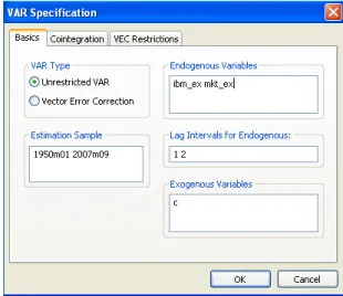
There are several ways to estimate VAR model in EViews. The first one is through the main menu. Clicking on View/Estimate VAR... will open a dialog window for VAR model estimation.

Figure 6.1: VAR model estimation dialog window

We choose Unrestricted VAR and in the Endogenous Variables box we have to specify the list of endogenous time series variables to be included in the VAR model. We consider two excess return series of the IBM stockIBM_exand the market portfolioMkt_ex.

In the Lag Intervals for Endogenous we have to specify the order of the model, that is interval of lags to be included in the model. If we want to build a model with only two lags, we write 1 2. This means, we include all lags beginning from the first one and ending with the lag of order 2. We do not specify any exogenous variables apart from the intercept term c.

Another way of calling the VAR estimation dialog window is to select both endogenous variables in the workfile and in the context menu (right button click) chooseOpen/as VAR.... TheEndogenous Variables box will be filled in auto- matically.

Finally, we can estimate VAR model from the command line. There is a separate object, calledvar, to declare the VAR model. The estimation of the above mentioned example will look like

100

(7)

101

var ibm2.ls 1 2 ibm_ex mkt_ex

Hereibm2is a name of the var-object which will be saved in the workfile,lsindicates the estimation method; in this case it is OLS estimation method of the unrestricted VAR model. Then, specifications of the lags pairs and the list of endogenous variables follow. If one wishes to include exogenous variables besides the intercept, it can be done by typing a symbol @ followed by a list of exogenous variables. For example,

var ibm2.ls 1 2 ibm_ex mkt_ex @ exvar1 exvar2

ClickOKand EViews produces an estimation output for the specified VAR model.

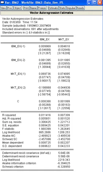
Figure 6.2: Output for the VAR model estimation

Two columns correspond to two equation in the VAR model. The only significant coefficient besides the intercept one is at the second lag of the market portfolio

101

(8)

returns in the IBM equation. As expected, there is a unidirectional dynamic relationship from the market portfolio returns to the IBM returns, Thus, the IBM return is affected by the past movements of the market while past movements of IBM stock returns do not affect the market portfolio returns. The second equation (for market portfolio) is not significant as suggested by the F-statistics. This means that the the estimated model cannot explain variation in the market portfolio returns. This can happen because we possibly omitted some important exogenous variables or the order of the model is inappropriately selected. EViews provides a tool to choose the most suitable lag order. In the workfile menu choose View/Lag Structure/Lag Length Criteria... to determine the optimal model structure. In the appeared Lag Specification window we choose pmax = 8 (maximal lag order).

All criteria indicate that the optimal lag order of the model is 0. This means that the VAR model is inappropriate model to explain IBM and market portfolio returns. Indeed, we know from the CAPM that market portfolio returns affect the stock returns contemporaneously and are not in lag relationship. Thus, either additional exogenous factors should be found to include in the model or another structure of the model should be employed in this case.

102

(9)

103

Figure 6.3: Output for the lag length selection procedure

Lag selection can be programmed manually in the same way as it is done for ARMA model (see Chapter 3). There are some command references given below which can be used to assess various statistic values in the VAR analysis in EViews.

6.2 Cointegration

The assumption of stationary of regressors and regressands is crucial for the proper- ties and the OLS estimators discussed in Chapter 2. In this case, the usual statistical results for the linear regression model and consistency of estimators hold. However, when variables are non-stationary then the usual statistical results may not hold.

6.2.1 Spurious Regression

If there are trends in the data (deterministic or stochastic) this can lead to a spurious results when running OLS regression. This is because time trend will dominate other stationary variables and the OLS estimators will pick up covariances generated by time trends only. While the effects of deterministic trends can be removed from the regression by either including time trend regressor or simply de-trending variables, non-stationary variables with stochastic trends may lead to invalid inferences.

103

(10)

104

Var Data Members

Data Member Description

@eqlogl(k) log likelihood for equation k

@eqncoef(k) number of estimated coefficients in equation k

@eqregobs(k) number of observations in equation k

@meandep(k) mean of the dependent variable in equation k

@r2(k) R-squared statistic for equation k

@rbar2(k) adjusted R-squared statistic for equation k

@sddep(k) standard deviation of dependent variable in equation k

@se(k) standard error of the regression in equation k

@ssr(k) sum of squared residuals in equation k

@aic Akaike information criterion for the system

@detresid determinant of the residual covariance matrix

@hq Hannan-Quinn information criterion for the system

@logl log likelihood for system

@ncoefs total number of estimated coefficients in the var

@neqn number of equations

@regobs number of observations in the var

@sc Schwarz information criterion for the system

@svarcvgtype

Returns an integer indicating the convergence type of the structural decomposition estimation: 0 (convergence achieved), 2 (failure to improve), 3 (maximum iterations reached), 4 (no convergence-structural decomposition not estimated)

@svaroverid over-identification LR statistic from structural factorization

@totalobs sum of "@eqregobs" from each equation ("@regobs*@neqn")

@coefmat coefficient matrix (as displayed in output table)

@coefse matrix of coefficient standard errors (corresponding to the output table)

@impfact factorization matrix used in last impulse response view

@lrrsp accumulated long-run responses from last impulse response view

@lrrspse standard errors of accumulated long-run responses

@residcov covariance matrix of the residuals

@svaramat estimated A matrix for structural factorization

@svarbmat estimated B matrix for structural factorization

@svarcovab covariance matrix of stacked A and B matrix for structural factorization

@svarrcov restricted residual covariance matrix from structural factorization

Consider, for example,

Y1,t =Y_1,t−1 +u1,t, u1,t ∼IN(0,1) Y2,t =Y2,t−1 +u2,t, u2,t ∼IN(0,1)

Both of the variables are non-stationary and independent from each other. In the regression Y1,t = β0+β1Y2,t+εt, the value of true slope parameter β1 = 0. Thus, the value of the OLS estimate βˆ1 should be insignificant. The actual estimations produce highR² coefficients and highly significantβ1.

The problem with the spurious regression is that t- and F-statistics do not follow standard distributions. As shown in Phillips (1986), βˆ1 does not converge in

104

(11)

probability to zero, R² converges to unity as T → ∞so that the model will appear to fit well even though it is misspecified.

Regression with I(1) data only makes sense when the data arecointegrated.

6.2.2 Cointegration

LetYt= (Y1t, ..., Ykt) denote ank×1 vector of I(1) time series. Yt is cointegrated if there exists ank×1 vectorβ = (β1, ..., βk) such that

Zt=βYt =β1Y1t+...+βkYkt∼I(0). (6.2.1) The non-stationary time series inYtare cointegrated if there is a linear combination of them that is stationary. If some elements of β are equal to zero then only the subset of the time series inYt with non-zero coefficients is cointegrated.

There may be different vectorsβsuch thatZt =βYtis stationary. In general, there can be0< r < klinearly independent cointegrating vectors. All cointegrating vectors form a cointegrating matrix B. This matrix is again not unique. Some normalization assumption is required to eliminate ambiguity from the definition.

105

EXPERIENCE THE POWER OF FULL ENGAGEMENT…

RUN FASTER.

RUN LONGER..

RUN EASIER…

READ MORE & PRE-ORDER TODAY WWW.GAITEYE.COM Challenge the way we run

1349906_A6_4+0.indd 1 22-08-2014 12:56:57

(12)

106

A typical normalization is

β= (1,−β2, ...,−βk)

so that the cointegration relationship may be expressed as Zt=βYt=Y1t−β2Y2t−...−βkYkt∼I(0).

6.2.3 Error Correction Models

Engle and Granger (1987) state that if a bivariateI(1)vectorYt= (Y1t, Y2t) is cointegrated with cointegrating vectorβ = (1,−β2) then there exists an error correction model (ECM) of the form

∆Y1t=δ1+φ1(Y1,t−1−β1Y2,t−1 +

j=1

α^j₁₁∆Y1,t−j+

s=1

α^j₁₂∆Y2,t−j+ε1t (6.2.2)

∆Y2t=δ2+φ2(Y_1,t−1−β2Y_2,t−1 +

j=1

α^j₂₁∆Y_1,t−j+

s=1

α^j₂₂∆Y_2,t−j+ε2t (6.2.3)

that describes the long-term relations of Y1t and Y2t. If both time series are I(1) but are cointegrated (have a long-term stationary relationship), there is a force that brings the error term back towards zero. If the cointegrating parameter β₁ or β₂ is known, the model can be estimated by the OLS method.

6.2.4 Tests for Cointegration: The Engle-Granger Approach

Engle and Granger (1987) show that if there is a cointegrating vector, a simple two-step residual-based testing procedure can be employed to test for cointegration.

In this case, a long-run equilibrium relationship between components of Yt can be estimated by running

Y1,t =βY2,t+ut, (6.2.4)

whereY_2,t= (Y_2,t, ..., Y_k,t) is an(k−1)×1 vector. To test the null hypothesis that Y_t is not cointegrated, we should test whether the residuals uˆ_t ∼ I(1) against the alternative uˆt ∼ I(0). This can be done by any of the tests for unit roots. The most commonly used is the augmented Dickey-Fuller test with the constant term and without the trend term. Critical values for this test is tabulated in Phillips and Ouliaris (1990) or MacKinnon (1996).

Potential problems with Engle-Granger approach is that the cointegrating vector will not involveY1,t component. In this case the cointegrating vector will not be consistently estimated from the OLS regression leading to spurious results. Also, if

106

(13)

there are more than one cointegrating relation, the Engle-Granger approach cannot detect all of them.

Estimation of the static model (6.2.4) is equivalent to omitting the short-term components from the error-correction model (6.2.3). If this results for autocorrela- tion in residuals, although the results will still hold asymptotically, it might create a severe bias in finite samples. Because of this, it makes sense to estimate the full dynamic model. Since all variables in the ECM areI(0), the model can be consistently estimated using the OLS method. This approach leads to a better performance as it does not push the short-term dynamics into residuals.

6.2.5 Example in EViews: Engle-Granger Approach

Consider as an example the Forward Premium Puzzle. Due to rational expectation hypothesis, forward rate should be unbiased predictor of future spot exchange rate.

This means that in the regression of levels of spot S_t+1 on forward rate F_t the intercept coefficient should be equal to zero and the slope coefficient should be equal to unity.

Consider monthly data of the USG/GBP spot and forward exchange rate for the period from January 1986 to November 2008 (the data is in FPP.wf1 file).

107

(14)

108

Unit roots are often found in in levels of spot and forward exchange rates.

Augmented Dickey-Fuller test statistic values are -2.567 and -2.688 which are high enough to fail rejecting the null hypothesis at 5%significance level. Phillips-Perron test produces test statistic which value os on the border of the rejection region.

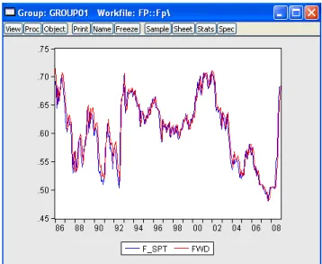
Thus, if two series are not cointegrated, there is a danger to obtain spurious results from the OLS regression. However, if we look at plots of the two series we can see that they co-move together very closely, so we can expect existence of cointegrating relation between them.

Figure 6.4: Plots of forward and future spot USD/GBP exchange rates

To perform Engle-Granger test for cointegration let us run OLS regression St+1 =βFt+ut in EViews and generate residuals from the model.

ls f_spt fwd series resid1=resid

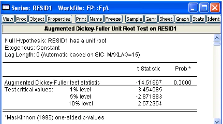
The second step is to test the residuals for stationarity. Augmented Dickey-Fuller test strongly rejects the presence of a unit root in the residual series in the favour of stationarity hypothesis.

Similar results are generated by other testing procedures. Thus, we conclude that future spot and forward exchange rates are cointegrated. Hence, the OLS results are valid for the regression in levels as well. In this case the slope coefficient is equal to 0.957 which is positive and close to unity. However, we reject the null hypothesisH0: β1 = 1 with the Wald test.

Thus, the forward premium puzzle also exists even for the model in levels for the exchange rates.

108

(15)

109

Figure 6.5: Results of Augmented Dickey-Fuller test for residuals from the long- run equilibrium relationship

Figure 6.6: Wald test results for testingH₀:β₁= 1

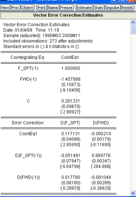
Another way of estimating cointegrating equation is to estimate a vector error correction model. To do this, open both forward and spot series as VAR system (select both series and in the context menu choose Open/as VAR...). In the VAR type box selectVector Error Correctionand in the Cointegration tab click on Intercept (no trend) in CE - no intercept in VAR. EViews’ output is given in Figure ??.

As expected, the output shows that the stationary series is approximately St+1 −Ft with the mean around zero. Deviations from the long-run equilibrium equation have significant effect on changes of the spot exchange rate. Another highly significant coefficient α¹₂₂ indicates a significant impact of∆St on∆Ft which is not surprising. This underlies the relationships between the spot and forward rate through the Covered Interest rate Parity condition (CIP).

The following subsection introduces an approach of testing for cointegration 109

(16)

110

Figure 6.7: Output of the vector error correction model

when there exists more than one cointegrating relationship.

6.2.6 Tests for Cointegration: The Johansen’s Approach

An alternative approach to test for cointegration was introduced by Johansen (1988).

His approach allows to avoid some drawbacks existing in the Engle-Granger’s approach and test the number of cointegrating relations directly. The method is based on the VAR model estimation.

Consider the V AR(p) model for the k×1vector Y_t

Y_t= Π₁Y_t−1 +...+ Π_pY_t−p +u_t, t= 1, ..., T, (6.2.5) whereut∼IN(0,Σ).

Since levels of time seriesYt might be non-stationary, it is better to transform Equation (6.2.5) into a dynamic form, calling vector error correction model (VECM)

∆Yt= ΠYt−1+ Γ1∆Yt−1+...+ Γp−1∆Yt−p+1+ut, whereΠ = Π1+...+ Πp −In and Γk=−

p j=k+1

Πj,k = 1, ..., p−1. 110

(17)

Let us assume that Yt contains non-stationary I(1) time series components.

Then in order to get a stationary error term ut, ΠYt−1 should also be stationary.

Therefore,ΠY_t−1must containr < k cointegrating relations. If theV AR(p)process has unit roots then Π has reduced rank rank(Π) = r < k. Effectively, testing for cointegration is equivalent to checking out the rank of the matrix Π.

IfΠ has a full rank then all time series inY are stationary, if the rank ofΠ is zero then there are no cointegrating relationships.

If 0<rank (Π) =r < k. This implies that Yt is I(1) with r linearly independent cointegrating vectors and k−r non-stationary vectors. Since Π has rank r it can be written as the product

(kΠ×k)= α

(k×r) β

(r×k)

,

where α and β are k ×r matrices with rank(α) = rank(β) = r. The matrix β is a matrix of long-run coefficients and α represents the speed of adjustment to disequilibrium. The VECM model becomes

∆Yt=αβYt−1+ Γ1Yt−1+...+ Γp−1∆Yt−p+1+ut, (6.2.6) with βY_t−1 ∼I(0).

111

www.sylvania.com

We do not reinvent the wheel we reinvent light.

Fascinating lighting offers an infinite spectrum of possibilities: Innovative technologies and new markets provide both opportunities and challenges.

An environment in which your expertise is in high demand. Enjoy the supportive working atmosphere within our global group and benefit from international career paths. Implement sustainable ideas in close cooperation with other specialists and contribute to influencing our future. Come and join us in reinventing light every day.

Light is OSRAM

(18)

112

Johansen’s methodology of obtaining estimates of α and β is given below.

Johansen’s Methodology

Specify and estimate a V AR(p)model (6.2.5) for Yt.

Determine the rank of Π; the maximum likelihood estimate for β equals the matrix of eigenvectors corresponding to ther largest eigenvalues of a k×k residual matrix (see Hamilton (1994), Lutkepohl (1991), Harris (1995) for more detailed description).

Construct likelihood ratio statistics for the number of cointegrating relationships. Let estimated eigenvalues areλˆ1 >λˆ2 > ... >λˆk of the matrix Π.

Johansen’s likelihood ratio statistic tests the nested hypotheses H0: r≤r0 vs. H1:r > r0

The likelihood ratio statistic, called thetrace statistic, is given by

LRtrace(r0) = −T k

i=r0+1

log 1−ˆλi

.

It checks whether the smallestk−r0 eigenvalues are statistically different from zero.

Ifrank (Π) =r0 then λˆr0+1, ...,ˆλk should all be close to zero and LRtrace(r0) should be small. In contrast, ifrank (Π) > r0 then some ofλˆr0+1, ...,λˆk will be nonzero (but less than 1) andLRtrace(r0) should be large.

We can also test H0: r = r₀ against H₁: r₀ = r₀ + 1 using so called the maximum eigenvalue statistic

LRmax(r0) =−T log

1−ˆλr0+1

.

Critical values for the asymptotic distribution ofLRtrace(r0)andLRmax(r0)statistics are tabulated in Osterwald-Lenum (1992) fork−r0 = 1, ...,10.

In order to determine the number of cointegrating vectors, first testH₀: r₀ = 0 against the alternative H₁: r₀ > 0. If this null is not rejected then it is concluded that there are no cointegrating vectors among thek variables inYt. If H0: r0 = 0 is rejected then there is at least one cointegrating vector. In this case we should test H0: r0 ≤ 1 against H1: r0 > 1. If this null is not rejected then we say that there is only one cointegrating vector. If the null is rejected then there are at least two cointegrating vectors. We testH0: r0 ≤2and so on until the null hypothesis is not rejected.

In a small samples tests are biased if asymptotic critical values are used without a correction. Reinsel and Ahn (1992) and Reimars (1992) suggested small samples bias correction by multiplying the test statistics with T −kp instead of T in the construction of the likelihood ratio tests.

112

(19)

113

6.2.7 Example in EViews: Johansen’s Approach

A very good example of a model with several cointegrating equations has been given by Johansen and Juselius (1990) (1992) (see also Harris (1995)). They considered a single equation approach to combine both Purchasing Power Parity and Uncovered Interest rate Parity condition in one model.

In this model we expect two cointegrating equations between the UK consumer price index P, the US consumer price index P^∗, USD/GBP exchange rate S and two interest ratesI and I^∗ in the domestic and foreign countries respectively. If we denote their log counterparts by the corresponding small letter, the theory suggest that the following two relationships should hold in efficient markets with rational investors: pt−p^∗_t =st and ∆st+1 =it−i^∗_t. The data is considered within the range from January 1989 to November 2008 is given in PPPFP1.wf1 file.

We create the log counterparts of the variables in the standard ways, like series lcpi_uk=log(cpi_uk)

and so on. In order to check for cointegration we can either estimate VECM (open 5 series as VAR model) or create a Group with the variables. Johansen and Juselius (1990) included into the model seasonal dummy variables as well as crude oil prices. We restrict ourself with only seasonal dummy for simplicity. We can create dummy variables by using a command @expand, which allows to create a group of dummy variables by expanding out one or more series into individual categories.

For this purposes we need first to create a variable indicating the quarter of the observation. We do it in the following way

series quarter=@quarter(cpi_uk)

The command @quarter returns the quarter of the year in which the current observation begins. The second step is to create the dummy variables:

group dum=@expand(quarter)

EViews will create a new group object dum containing four dummy variables for each of the quarter of the observation.

In both cases, either with VAR or with group objects, one can perform Jo- hansen’s test procedure by clicking on View/Cointegration Test....

The dialog window will ask offer to specify the form of the VECM and the cointegrating equation (with or without intercept or trend components). We choose the first option with no trend and intercept to avoid perfect collinearity since we include four dummy variables as exogenous in the model. In the box Exogenous Variablesenter the name of the dummy variables group dum.

In the boxLag Intervals for D(Endogenous)we set1 4– we include 4 lags 113

(20)

Figure 6.8: Johansen’s Cointegration test dialog window

in the model. This is determined by EViews as optimal according to 3 criteria (first estimate VAR with any of the lag specifications, check the optimality of the lag order in View/Lag Structure/Lag Specification/Lag Length Criteria and then re-estimate the VECM with the optimal lag order).

114

360° thinking .

Discover the truth at www.deloitte.ca/careers

360° thinking .

Discover the truth at www.deloitte.ca/careers

360° thinking .

Discover the truth at www.deloitte.ca/careers

360° thinking .

Discover the truth at www.deloitte.ca/careers

(21)

115

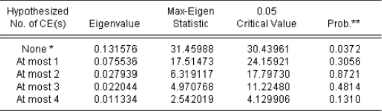
Figure 6.9: Output for Johansen’s Cointegration test

EViews produces results for various hypothesis tested, from no cointegration (r = 0) to to increasing number of cointegrating vectors (see Figure ??). The eigenvalues of matrix Πˆ is given in the second column. In the third column λ_trace statistic is higher than the corresponding critical value at 5% significance for the first hypothesis. This means that we reject the null hypothesis of no cointegration.

115

(22)

116

However, we cannot reject the hypothesis that there is at most one cointegrating equation. On the basis of λmax statistics (the second panel) it is also possible to accept that there is only one cointegrating relationship. The following two panels provide estimates of matrices β and α respectively.

Note the warning on the top of the output window that saying that critical values assume no exogenous series. This means that we have to take into account that the critical values we are using might not be fully correct as we included exogenous dummy variables in the model. This may give as an explanation why we detected only one cointegrating equation instead of two which were expected. An- other reason may be that the second relation based on the UIP condition involves changes of exchange rate rather than levels considered in the VAR model.

116