Analysis of Financial Time Series

(1)

(2)

Analysis of Financial Time Series

Second Edition

RUEY S. TSAY

University of Chicago Graduate School of Business

(3)

(4)

(5)

Established by WALTER A. SHEWHART and SAMUEL S. WILKS

Editors:David J. Balding, Noel A. C. Cressie, Nicholas I. Fisher,

Iain M. Johnstone, J. B. Kadane, Geert Molenberghs, Louise M. Ryan, David W. Scott, Adrian F. M. Smith, Jozef L. Teugels

Editors Emeriti:Vic Barnett, J. Stuart Hunter, David G. Kendall

(6)

Analysis of Financial Time Series

Second Edition

RUEY S. TSAY

University of Chicago Graduate School of Business

(7)

Published by John Wiley & Sons, Inc., Hoboken, New Jersey. Published simultaneously in Canada.

No part of this publication may be reproduced, stored in a retrieval system, or transmitted in any form or by any means, electronic, mechanical, photocopying, recording, scanning, or otherwise, except as permitted under Section 107 or 108 of the 1976 United States Copyright Act, without either the prior written permission of the Publisher, or authorization through payment of the appropriate per-copy fee to the Copyright Clearance Center, Inc., 222 Rosewood Drive, Danvers, MA 01923, (978) 750-8400, fax (978) 750-4470, or on the web at www.copyright.com. Requests to the Publisher for permission should be addressed to the Permissions Department, John Wiley & Sons, Inc., 111 River Street, Hoboken, NJ 07030, (201) 748-6011, fax (201) 748-6008, or online at

http://www.wiley.com/go/permission.

Limit of Liability/Disclaimer of Warranty: While the publisher and author have used their best efforts in preparing this book, they make no representations or warranties with respect to the accuracy or completeness of the contents of this book and specifically disclaim any implied warranties of merchantability or fitness for a particular purpose. No warranty may be created or extended by sales representatives or written sales materials. The advice and strategies contained herein may not be suitable for your situation. You should consult with a professional where appropriate. Neither the publisher nor author shall be liable for any loss of profit or any other commercial damages, including but not limited to special, incidental, consequential, or other damages.

For general information on our other products and services or for technical support, please contact our Customer Care Department within the United States at (800) 762-2974, outside the United States at (317) 572-3993 or fax (317) 572-4002.

Wiley also publishes its books in a variety of electronic formats. Some content that appears in print may not be available in electronic formats. For more information about Wiley products, visit our web site at www.wiley.com.

Library of Congress Cataloging-in-Publication Data:

Tsay, Ruey S., 1951–

Analysis of ﬁnancial time series/Ruey S. Tsay.—2nd ed. p. cm.

“Wiley-Interscience.”

Includes bibliographical references and index. ISBN-13 978-0-471-69074-0

ISBN-10 0-471-69074-0 (cloth)

1. Time-series analysis. 2. Econometrics. 3. Risk management. I. Title. HA30.3T76 2005

332′_.01′_51955—dc22

2005047030 Printed in the United States of America.

(8)

(9)

(10)

Preface

The subject of financial time series analysishas attracted substantial attention in recent years, especially with the 2003 Nobel awards to Professors Robert Engle and Clive Granger. At the same time, the field of financial econometrics has undergone various new developments, especially in high-frequency finance, stochastic volatil-ity, and software availability. There is a need to make the material more complete and accessible for advanced undergraduate and graduate students, practitioners, and researchers. The main goals in preparing this second edition have been to bring the book up to date both in new developments and empirical analysis, and to enlarge the core material of the book by including consistent covariance estimation under heteroscedasticity and serial correlation, alternative approaches to volatility mod-eling, financial factor models, state-space models, Kalman filtering, and estimation of stochastic diffusion models.

The book therefore has been extended to 10 chapters and substantially revised to include S-Plus commands and illustrations. Many empirical demonstrations and exercises are updated so that they include the most recent data.

The two new chapters are Chapter 9, Principal Component Analysis and Factor Models, and Chapter 11, State-Space Models and Kalman Filter. The factor mod-els discussed include macroeconomic, fundamental, and statistical factor modmod-els. They are simple and powerful tools for analyzing high-dimensional financial data such as portfolio returns. Empirical examples are used to demonstrate the appli-cations. The state-space model and Kalman filter are added to demonstrate their applicability in finance and ease in computation. They are used in Chapter 12 to estimate stochastic volatility models under the general Markov chain Monte Carlo (MCMC) framework. The estimation also uses the technique of forward filtering and backward sampling to gain computational efficiency.

A brief summary of the added material in the second edition is:

1. To update the data used throughout the book.

2. To provide S-Plus commands and demonstrations.

3. To consider unit-root tests and methods for consistent estimation of the covariance matrix in the presence of conditional heteroscedasticity and serial correlation in Chapter 2.

(21)

4. To describe alternative approaches to volatility modeling, including use of high-frequency transactions data and daily high and low prices of an asset in Chapter 3.

5. To give more applications of nonlinear models and methods in Chapter 4.

6. To introduce additional concepts and applications of value at risk in Chapter 7.

7. To discuss cointegrated vector AR models in Chapter 8.

8. To cover various multivariate volatility models in Chapter 10.

9. To add an effective MCMC method for estimating stochastic volatility models in Chapter 12.

The revision benefits greatly from constructive comments of colleagues, friends, and many readers on the first edition. I am indebted to them all. In particular, I thank J. C. Artigas, Spencer Graves, Chung-Ming Kuan, Henry Lin, Daniel Peña, Jeff Russell, Michael Steele, George Tiao, Mark Wohar, Eric Zivot, and students of my MBA classes on financial time series for their comments and discussions, and Rosalyn Farkas, production editor, at John Wiley. I also thank my wife and children for their unconditional support and encouragement. Part of my research in financial econometrics is supported by the National Science Foundation, the High-Frequency Finance Project of the Institute of Economics, Academia Sinica, and the Graduate School of Business, University of Chicago.

Finally, the website for the book is:

gsbwww.uchicago.edu/fac/ruey.tsay/teaching/fts2.

Ruey S. Tsay University of Chicago

(22)

Preface for the First Edition

This book grew out of an MBA course in analysis of financial time series that I have been teaching at the University of Chicago since 1999. It also covers materials of Ph.D. courses in time series analysis that I taught over the years. It is an introductory book intended to provide a comprehensive and systematic account of financial econometric models and their application to modeling and prediction of financial time series data. The goals are to learn basic characteristics of financial data, understand the application of financial econometric models, and gain experience in analyzing financial time series.

The book will be useful as a text of time series analysis for MBA students with finance concentration or senior undergraduate and graduate students in business, economics, mathematics, and statistics who are interested in financial econometrics. The book is also a useful reference for researchers and practitioners in business, finance, and insurance facing value at risk calculation, volatility modeling, and analysis of serially correlated data.

The distinctive features of this book include the combination of recent devel-opments in ﬁnancial econometrics in the econometric and statistical literature. The developments discussed include the timely topics of value at risk (VaR), high-frequency data analysis, and Markov chain Monte Carlo (MCMC) methods. In particular, the book covers some recent results that are yet to appear in academic journals; see Chapter 6 on derivative pricing using jump diffusion with closed-form closed-formulas, Chapter 7 on value at risk calculation using extreme value theory based on a nonhomogeneous two-dimensional Poisson process, and Chapter 9 on multivariate volatility models with time-varying correlations. MCMC methods are introduced because they are powerful and widely applicable in ﬁnancial economet-rics. These methods will be used extensively in the future.

Another distinctive feature of this book is the emphasis on real examples and data analysis. Real ﬁnancial data are used throughout the book to demonstrate applications of the models and methods discussed. The analysis is carried out by using several computer packages; the SCA (the Scientiﬁc Computing Associates)

(23)

for building linear time series models, the RATS (regression analysis for time series) for estimating volatility models, and the S-Plus for implementing neural networks and obtaining postscript plots. Some commands required to run these packages are given in appendixes of appropriate chapters. In particular, complicated RATS programs used to estimate multivariate volatility models are shown in Appendix A of Chapter 9. Some Fortran programs written by myself and others are used to price simple options, estimate extreme value models, calculate VaR, and carry out Bayesian analysis. Some data sets and programs are accessible from the World Wide Web at http://www.gsb.uchicago.edu/fac/ruey.tsay/teaching/fts.

The book begins with some basic characteristics of financial time series data in Chapter 1. The other chapters are divided into three parts. The first part, consisting of Chapters 2 to 7, focuses on analysis and application of univariate financial time series. The second part of the book covers Chapters 8 and 9 and is concerned with the return series of multiple assets. The final part of the book is Chapter 10, which introduces Bayesian inference in finance via MCMC methods.

A knowledge of basic statistical concepts is needed to fully understand the book. Throughout the chapters, I have provided a brief review of the necessary statistical concepts when they first appear. Even so, a prerequisite in statistics or business statistics that includes probability distributions and linear regression analysis is highly recommended. A knowledge of finance will be helpful in understanding the applications discussed throughout the book. However, readers with advanced back-ground in econometrics and statistics can find interesting and challenging topics in many areas of the book.

An MBA course may consist of Chapters 2 and 3 as a core component, followed by some nonlinear methods (e.g., the neural network of Chapter 4 and the applica-tions discussed in Chapters 5–7 and 10). Readers who are interested in Bayesian inference may start with the ﬁrst ﬁve sections of Chapter 10.

Research in ﬁnancial time series evolves rapidly and new results continue to appear regularly. Although I have attempted to provide broad coverage, there are many subjects that I do not cover or can only mention in passing.

(24)

PREFACE FOR THE FIRST EDITION xxi

understanding; to Julie, Richard, and Vicki for bringing me joy and inspirations; and to my parents for their love and care.

Ruey S. Tsay University of Chicago

(25)

(26)

C H A P T E R 1

Financial Time Series and

Their Characteristics

Financial time series analysis is concerned with the theory and practice of asset valuation over time. It is a highly empirical discipline, but like other scientific fields theory forms the foundation for making inference. There is, however, a key feature that distinguishes financial time series analysis from other time series analysis. Both financial theory and its empirical time series contain an element of uncertainty. For example, there are various definitions of asset volatility, and for a stock return series, the volatility is not directly observable. As a result of the added uncertainty, statistical theory and methods play an important role in financial time series analysis.

The objective of this book is to provide some knowledge of financial time series, introduce some statistical tools useful for analyzing these series, and gain experience in financial applications of various econometric methods. We begin with the basic concepts of asset returns and a brief introduction to the processes to be discussed throughout the book. Chapter 2 reviews basic concepts of linear time series analysis such as stationarity and autocorrelation function, introduces simple linear models for handling serial dependence of the series, and discusses regression models with time series errors, seasonality, unit-root nonstationarity, and long-memory processes. The chapter also provides methods for consistent estima-tion of the covariance matrix in the presence of condiestima-tional heteroscedasticity and serial correlations. Chapter 3 focuses on modeling conditional heteroscedasticity (i.e., the conditional variance of an asset return). It discusses various economet-ric models developed recently to describe the evolution of volatility of an asset return over time. The chapter also discusses alternative methods to volatility mod-eling, including use of high-frequency transactions data and daily high and low prices of an asset. In Chapter 4, we address nonlinearity in financial time series, introduce test statistics that can discriminate nonlinear series from linear ones, and discuss several nonlinear models. The chapter also introduces nonparametric Analysis of Financial Time Series, Second Edition By Ruey S. Tsay

Copyright_{2005 John Wiley & Sons, Inc.}

(27)

estimation methods and neural networks and shows various applications of non-linear models in finance. Chapter 5 is concerned with analysis of high-frequency financial data and its application to market microstructure. It shows that nonsyn-chronous trading and bid–ask bounce can introduce serial correlations in a stock return. It also studies the dynamic of time duration between trades and some econometric models for analyzing transactions data. In Chapter 6, we introduce continuous-time diffusion models and Ito’s lemma. Black–Scholes option pric-ing formulas are derived and a simple jump diffusion model is used to capture some characteristics commonly observed in options markets. Chapter 7 discusses extreme value theory, heavy-tailed distributions, and their application to financial risk management. In particular, it discusses various methods for calculating value at risk of a financial position. Chapter 8 focuses on multivariate time series anal-ysis and simple multivariate models with emphasis on the lead–lag relationship between time series. The chapter also introduces cointegration, some cointegra-tion tests, and threshold cointegracointegra-tion and applies the concept of cointegracointegra-tion to investigate arbitrage opportunity in financial markets. Chapter 9 discusses ways to simplify the dynamic structure of a multivariate series and methods to reduce the dimension. It introduces and demonstrates three types of factor model to ana-lyze returns of multiple assets. In Chapter 10, we introduce multivariate volatility models, including those with time-varying correlations, and discuss methods that can be used to reparameterize a conditional covariance matrix to satisfy the pos-itiveness constraint and reduce the complexity in volatility modeling. Chapter 11 introduces state-space models and the Kalman filter and discusses the relationship between state-space models and other econometric models discussed in the book. It also gives several examples of financial applications. Finally, in Chapter 12, we introduce some newly developed Markov chain Monte Carlo (MCMC) meth-ods in the statistical literature and apply the methmeth-ods to various financial research problems, such as the estimation of stochastic volatility and Markov switching models.

The book places great emphasis on application and empirical data analysis. Every chapter contains real examples and, on many occasions, empirical character-istics of ﬁnancial time series are used to motivate the development of econometric models. Computer programs and commands used in data analysis are provided when needed. In some cases, the programs are given in an appendix. Many real data sets are also used in the exercises of each chapter.

1.1 ASSET RETURNS

(28)

ASSET RETURNS 3

LetPt be the price of an asset at time indext. We discuss some deﬁnitions of returns that are used throughout the book. Assume for the moment that the asset pays no dividends.

One-Period Simple Return

Holding the asset for one period from datet−1 to datet would result in asimple gross return

1+Rt = Pt Pt−1

or Pt =Pt−1(1+Rt). (1.1)

The corresponding one-periodsimple net returnor simple returnis

Rt =

Holding the asset fork periods between datest−k andt gives ak-period simple gross return

Thus, thek-period simple gross return is just the product of thekone-period simple gross returns involved. This is called a compound return. Thek-period simple net return isRt[k]=(Pt−Pt−k)/Pt−k.

In practice, the actual time interval is important in discussing and comparing returns (e.g., monthly return or annual return). If the time interval is not given, then it is implicitly assumed to be one year. If the asset was held forkyears, then the annualized (average) return is deﬁned as

Annualized{Rt[k]} =

This is a geometric mean of the k one-period simple gross returns involved and can be computed by

Annualized{R_t[k]} =exp

(29)

geometric mean and the one-period returns tend to be small, one can use a ﬁrst-order Taylor expansion to approximate the annualized return and obtain

Annualized{Rt[k]} ≈ 1 k

k−1

j=0

Rt−j. (1.3)

Accuracy of the approximation in Eq. (1.3) may not be sufﬁcient in some applica-tions, however.

Continuous Compounding

Before introducing continuously compounded return, we discuss the effect of com-pounding. Assume that the interest rate of a bank deposit is 10% per annum and the initial deposit is $1.00. If the bank pays interest once a year, then the net value of the deposit becomes $1(1₊0.1)₌$1.1 one year later. If the bank pays interest semiannually, the 6-month interest rate is 10%/2₌5% and the net value is $1(1₊0.1/2)2₌$1.1025 after the ﬁrst year. In general, if the bank pays interest mtimes a year, then the interest rate for each payment is 10%/mand the net value of the deposit becomes $1(1+0.1/m)m _{one year later. Table 1.1 gives the results} for some commonly used time intervals on a deposit of $1.00 with interest rate of 10% per annum. In particular, the net value approaches $1.1052, which is obtained by exp(0.1)and referred to as the result of continuous compounding. The effect of compounding is clearly seen.

In general, the net asset valueAof continuous compounding is

A₌Cexp(r_×n), (1.4)

whereris the interest rate per annum,C is the initial capital, andnis the number of years. From Eq. (1.4), we have

C₌Aexp(₋r_×n), (1.5)

which is referred to as thepresent valueof an asset that is worthAdollarsnyears from now, assuming that the continuously compounded interest rate isrper annum.

Table 1.1. Illustration of the Effects of Compoundinga

Number of Interest Rate

Type Payments per Period Net Value

Annual 1 0.1 $1.10000

Semiannual 2 0.05 $1.10250

Quarterly 4 0.025 $1.10381

Monthly 12 0.0083 $1.10471

Weekly 52 0.1/52 $1.10506

Daily 365 0.1/365 $1.10516

Continuously ∞ $1.10517

(30)

ASSET RETURNS 5

Continuously Compounded Return

The natural logarithm of the simple gross return of an asset is called the continu-ously compounded return orlog return:

rt =ln(1+Rt)=ln Pt Pt−1 =

pt −pt−1, (1.6)

where pt = ln(Pt). Continuously compounded returns rt enjoy some advantages over the simple net returnsRt. First, consider multiperiod returns. We have

rt[k]=ln(1+Rt[k])=ln[(1+Rt)(1+Rt−1)· · ·(1+Rt−k+1)]

=ln(1₊Rt)+ln(1+Rt−1)+ · · · +ln(1+Rt−k+1)

=rt+rt−1+ · · · +rt−k+1.

Thus, the continuously compounded multiperiod return is simply the sum of con-tinuously compounded one-period returns involved. Second, statistical properties of log returns are more tractable.

Portfolio Return

The simple net return of a portfolio consisting of N assets is a weighted average of the simple net returns of the assets involved, where the weight on each asset is the percentage of the portfolio’s value invested in that asset. Let pbe a portfolio that places weight wi on asset i. Then the simple return ofp at timet is Rp,t= N

i=1wiRit, whereRit is the simple return of asseti.

The continuously compounded returns of a portfolio, however, do not have the above convenient property. If the simple returnsRit are all small in magnitude, then

we have rp,t≈Ni=1wirit, where rp,t is the continuously compounded return of the portfolio at timet. This approximation is often used to study portfolio returns.

Dividend Payment

If an asset pays dividends periodically, we must modify the deﬁnitions of asset returns. LetDt be the dividend payment of an asset between datest−1 andt and Pt be the price of the asset at the end of periodt. Thus, dividend is not included inPt. Then the simple net return and continuously compounded return at time t become

Rt =

Pt+Dt

P_t−1 −1, rt=ln(Pt+Dt)−ln(Pt−1).

Excess Return

Excess return of an asset at timet is the difference between the asset’s return and the return on some reference asset. The reference asset is often taken to be riskless such as a short-term U.S. Treasury bill return. The simple excess return and log excess return of an asset are then deﬁned as

(31)

whereR0tandr0tare the simple and log returns of the reference asset, respectively. In the ﬁnance literature, the excess return is thought of as the payoff on an arbitrage portfolio that goes long in an asset and short in the reference asset with no net initial investment.

Remark. A long ﬁnancial position means owning the asset. A short position

involves selling an asset one does not own. This is accomplished by borrowing the asset from an investor who has purchased it. At some subsequent date, the short seller is obligated to buy exactly the same number of shares borrowed to pay back the lender. Because the repayment requires equal shares rather than equal dollars, the short seller beneﬁts from a decline in the price of the asset. If cash dividends are paid on the asset while a short position is maintained, these are paid to the buyer of the short sale. The short seller must also compensate the lender by matching the cash dividends from his own resources. In other words, the short seller is also obligated to pay cash dividends on the borrowed asset to the lender.

Summary of Relationship

The relationships between simple returnRt and continuously compounded (or log) returnrt are

rt =ln(1+Rt), Rt =ert −1.

If the returnsRt andrt are in percentages, then

rt =100 ln

1₊ Rt

100 , Rt =100(e rt/100

−1).

Temporal aggregation of the returns produces

1₊Rt[k]=(1+Rt)(1+Rt−1)· · ·(1+Rt−k+1), rt[k]=rt+rt−1+ · · · +rt−k+1.

If the continuously compounded interest rate isr per annum, then the relationship between present and future values of an asset is

A₌Cexp(r_×n), C₌Aexp(₋r_×n).

Example 1.1. If the monthly log return of an asset is 4.46%, then the

(32)

DISTRIBUTIONAL PROPERTIES OF RETURNS 7

1.2 DISTRIBUTIONAL PROPERTIES OF RETURNS

To study asset returns, it is best to begin with their distributional properties. The objective here is to understand the behavior of the returns across assets and over time. Consider a collection ofN assets held forT time periods, say,t ₌1,. . . , T. For each asset i, let rit be its log return at time t. The log returns under study

are _{rit;i=1, . . . , N;t =1, . . . , T}. One can also consider the simple returns {Rit;i=1, . . . , N;t=1, . . . , T} and the log excess returns {zit;i=1, . . . , N;

t ₌1, . . . , T_}.

1.2.1 Review of Statistical Distributions and Their Moments

We brieﬂy review some basic properties of statistical distributions and the moment equations of a random variable. Let Rk be the k-dimensional Euclidean space. A point inRkis denoted byx∈Rk. Consider two random vectorsX=(X1, . . . , Xk)′ andY ₌(Y1, . . . , Yq)′. Let P (X∈A,Y ∈B) be the probability thatX is in the subspaceA_⊂RkandY is in the subspaceB _⊂Rq. For most of the cases consid-ered in this book, both random vectors are assumed to be continuous.

Joint Distribution

The function

FX,Y(x,y;θ)=P (X≤x,Y ≤y;θ),

wherex_∈Rp,y_∈Rq, and the inequality “_≤” is a component-by-component oper-ation, is a joint distribution function ofXandY with parameterθ. Behavior ofX

and Y is characterized by F_X,Y(x,y_;θ). If the joint probability density function fx,y(x,y;θ)ofX andY exists, then

FX,Y(x,y;θ)= x

−∞ y

−∞

fx,y(w,z;θ) dzdw.

In this case,X andY are continuous random vectors.

Marginal Distribution

The marginal distribution ofX is given by

FX(x;θ)=FX,Y(x,∞, . . . ,∞;θ).

Thus, the marginal distribution of X is obtained by integrating outY. A similar deﬁnition applies to the marginal distribution ofY.

Ifk₌1, Xis a scalar random variable and the distribution function becomes FX(x)=P (X≤x;θ),

(33)

F_X(_−∞)₌0 andF_X(_∞)₌1. For a given probabilityp, the smallest real number xpsuch thatp≤FX(xp)is called thepth quantile of the random variableX. More speciﬁcally,

xp=inf

x {x|p≤FX(x)}.

We use the CDF to compute thep value of a test statistic in the book.

Conditional Distribution

The conditional distribution ofXgiven Y _≤y is given by

FX|Y≤y(x;θ)=

P (X_≤x,Y _≤y_;θ) P (Y ≤y;θ) .

If the probability density functions involved exist, then the conditional density of

X givenY =y is

fx|y(x;θ)=

fx,y(x,y;θ) fy(y;θ)

, (1.8)

where the marginal density functionfy(y;θ)is obtained by

fy(y;θ)= _∞

−∞

fx,y(x,y;θ) dx.

From Eq. (1.8), the relation among joint, marginal, and conditional distributions is

fx,y(x,y;θ)=fx|y(x;θ)×fy(y;θ). (1.9) This identity is used extensively in time series analysis (e.g., in maximum like-lihood estimation). Finally, X andY are independent random vectors if and only if f_x|y(x_;θ)₌fx(x;θ). In this case, fx,y(x,y;θ)=fx(x;θ)fy(y;θ).

Moments of a Random Variable

The ℓth moment of a continuous random variableXis deﬁned as

m′_ℓ₌E(Xℓ)₌

_∞

−∞

xℓf (x) dx,

whereEstands for expectation andf (x)is the probability density function ofX. The ﬁrst moment is called the mean or expectationof X. It measures the central location of the distribution. We denote the mean of X by µx. The ℓth central moment of X is deﬁned as

mℓ=E[(X−µx)ℓ]= ∞

−∞

(34)

provided that the integral exists. The second central moment, denoted byσ_x2, mea-sures the variability ofXand is called thevarianceofX. The positive square root, σx, of variance is thestandard deviationofX. The ﬁrst two moments of a random variable uniquely determine a normal distribution. For other distributions, higher order moments are also of interest.

The third central moment measures the symmetry ofXwith respect to its mean, whereas the fourth central moment measures the tail behavior of X. In statistics, skewness and kurtosis, which are normalized third and fourth central moments of X, are often used to summarize the extent of asymmetry and tail thickness. Speciﬁcally, the skewness and kurtosis ofX are deﬁned as

S(x)₌E

The quantityK(x)₋3 is called theexcess kurtosisbecauseK(x)₌3 for a normal distribution. Thus, the excess kurtosis of a normal random variable is zero. A distribution with positive excess kurtosis is said to have heavy tails, implying that the distribution puts more mass on the tails of its support than a normal distribution does. In practice, this means that a random sample from such a distribution tends to contain more extreme values. Such a distribution is said to be leptokurtic. On the other hand, a distribution with negative excess kurtosis has short tails (e.g., a uniform distribution over a ﬁnite interval). Such a distribution is said to be platykurtic.

In application, skewness and kurtosis can be estimated by their sample counter-parts. Let_{x1, . . . , xT}be a random sample ofX withT observations. The sample

the sample variance is

ˆ

the sample skewness is

ˆ

and the sample kurtosis is

ˆ

(35)

and Cochran (1980, p. 78). These asymptotic properties can be used to test the normality of asset returns. Given an asset return series _{r1, . . . , rT}, to test the skewness of the returns, we consider the null hypothesisHo:S(r)=0 versus the alternative hypothesisHa :S(r)=0. The t-ratio statistic of the sample skewness in Eq. (1.12) is

t ₌ _√S(r)ˆ 6/T.

The decision rule is as follows. Reject the null hypothesis at the α signiﬁcance level, if _|t_|> Zα/2, where Zα/2 is the upper 100(α/2)th quantile of the standard normal distribution. Alternatively, one can compute thep-value of the test statistic t and rejectHo if and only if thep-value is less thanα.

Similarly, one can test the excess kurtosis of the return series using the hypothe-ses Ho :K(r)−3=0 versusHa :K(r)−3=0. The test statistic is

t ₌K(r)_√ˆ −3 24/T ,

which is asymptotically a standard normal random variable. The decision rule is to rejectHo if and only if thep-value of the test statistic is less than the signiﬁcance level α. Jarque and Bera (1987) combine the two prior tests and use the test statistic

J B₌ Sˆ 2_(r) 6/T +

(K(r)ˆ ₋3)2 24/T ,

which is asymptotically distributed as a chi-squared random variable with 2 degrees of freedom, to test for the normality ofrt. One rejectsHoof normality if thep-value of theJ B statistic is less than the signiﬁcance level.

Example 1.2. Consider the daily simple returns of the IBM stock used in

Table 1.2. The sample skewness and kurtosis of the returns are parts of the descrip-tive (or summary) statistics that can be obtained easily using various statistical software packages. Both SCA and S-Plus are used in the demonstration, where ‘d-ibmvwewsp6203.txt’ is the data ﬁle name. Note that in SCA the kurtosis denotes excess kurtosis. From the output, the excess kurtosis is high, indicating that the daily simple returns of IBM stock have heavy tails. To test the symmetry of return distribution, we use the test statistic

t ₌ 0.0775

0.024 =3.23,

(36)

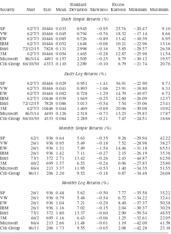
Table 1.2. Descriptive Statistics for Daily and Monthly Simple and Log Returns of Selected Indexes and Stocksa

Standard Excess

Security Start Size Mean Deviation Skewness Kurtosis Minimum Maximum

Daily Simple Returns (%)

SP 62/7/3 10446 0.033 0.945 −0.95 25.76 −20.47 9.10

VW 62/7/3 10446 0.045 0.794 −0.76 18.32 −17.14 8.66

EW 62/7/3 10446 0.085 0.726 −0.89 13.42 −10.39 6.95

IBM 62/7/3 10446 0.052 1.648 −0.08 10.21 −22.96 13.16

Intel 72/12/15 7828 0.131 2.998 −0.16 5.85 −29.57 26.38

3M 62/7/3 10446 0.054 1.465 −0.28 12.87 −25.98 11.54

Microsoft 86/3/14 4493 0.157 2.505 −0.25 8.75 −30.12 19.57

Citi-Group 86/10/30 4333 0.110 2.289 −0.10 6.79 −21.74 20.76

Daily Log Returns (%)

SP 62/7/3 10446 0.029 0.951 −1.41 36.91 −22.90 8.71

VW 62/7/3 10446 0.041 0.895 −1.06 23.91 −18.80 8.31

EW 62/7/3 10446 0.082 0.728 −1.29 14.70 −10.97 6.72

IBM 62/7/3 10446 0.039 1.649 −0.25 12.60 −26.09 12.37

Intel 72/12/15 7828 0.086 3.013 −0.54 7.54 −35.06 23.41

3M 62/7/3 10446 0.044 1.469 −0.69 20.06 −30.08 10.92

Microsoft 86/3/14 4493 0.126 2.518 −0.73 13.23 −35.83 17.87

Citi-Group 86/10/30 4333 0.084 2.289 −0.21 7.47 −24.51 18.86

Monthly Simple Returns (%)

SP 62/1 936 0.64 5.63 −0.35 9.26 −29.94 42.22

VW 26/1 936 0.95 5.49 −0.18 7.52 −28.98 38.27

EW 26/1 936 1.31 7.49 −1.54 14.46 −31.18 65.51

IBM 26/1 936 1.42 7.11 −0.27 2.15 −26.19 35.38

Intel 73/1 372 2.71 13.42 −0.26 2.43 −44.87 62.50

3M 46/2 695 1.37 6.53 −0.24 0.96 −27.83 25.80

Microsoft 86/4 213 3.37 11.95 −0.53 1.40 −34.35 51.55

Citi-Group 86/11 206 2.20 9.52 −0.18 0.87 −34.48 26.08

Monthly Log Returns (%)

SP 26/1 936 0.48 5.62 −0.50 7.77 −35.58 35.22

VW 26/1 936 0.79 5.48 −0.54 6.72 −34.22 32.41

EW 26/1 936 1.04 7.21 −0.29 8.40 −37.37 50.38

IBM 26/1 936 1.16 7.02 −0.15 2.04 −30.37 30.29

Intel 73/1 372 1.80 13.37 −0.60 2.90 −59.54 48.55

3M 46/2 695 1.16 6.43 −0.06 1.25 −32.61 22.95

Microsoft 86/4 213 2.66 11.48 −0.01 1.19 −42.09 41.58

Citi-Group 86/11 206 1.73 9.55 −0.65 2.08 −42.28 23.18

(37)

SCA Demonstration

% denotes explanation.

input date, ibm, vw, ew, sp. file ’d-ibmvwewsp6203.txt’ % Load data into SCA and name the columns date,

% ibm, vw, ew, and sp.

--ibm=ibm*100 % Compute percentage returns

--desc ibm % Obtain descriptive statistics of ibm

VARIABLE NAME IS IBM

NUMBER OF OBSERVATIONS 10446 NUMBER OF MISSING VALUES 0

STATISTIC STD. ERROR STATISTIC/S.E.

MEAN 0.0523 0.0161 3.2457

VARIANCE 2.7163

STD DEVIATION 1.6481

C.V. 31.4900

SKEWNESS 0.0775 0.0240

KURTOSIS 10.2144 0.0479

QUARTILE

MINIMUM -22.9630

1ST QUARTILE -0.8380

MEDIAN 0.0000

3RD QUARTILE 0.8805

MAXIMUM 13.1640

RANGE

MAX - MIN 36.1270

Q3 - Q1 1.7185

S-Plus Demonstration

>is the prompt character and % marks explanation.

> module(finmetrics) % Load the Finmetrics module.

> x=matrix(scan(file=’d-ibmvwewsp6203.txt’),5) % Load data > ibm=x[2,]*100 % compute percentage returns

> summaryStats(ibm) % obtain summary statistics Sample Quantiles:

min 1Q median 3Q max

-22.96 -0.838 0 0.8807 13.16 Sample Moments:

(38)

1.2.2 Distributions of Returns

The most general model for the log returns_{rit;i=1, . . . , N;t =1, . . . , T}is its

joint distribution function:

Fr(r11, . . . , rN1;r12, . . . , rN2;. . .;r1T, . . . , rNT;Y;θ), (1.14)

whereY is a state vector consisting of variables that summarize the environment in which asset returns are determined andθis a vector of parameters that uniquely determine the distribution functionFr(.). The probability distributionFr(.)governs the stochastic behavior of the returnsrit andY. In many ﬁnancial studies, the state

vectorY is treated as given and the main concern is the conditional distribution of

{rit}givenY. Empirical analysis of asset returns is then to estimate the unknown

parameterθand to draw statistical inference about the behavior of_{rit}given some

past log returns.

The model in Eq. (1.14) is too general to be of practical value. However, it provides a general framework with respect to which an econometric model for asset returns rit can be put in a proper perspective.

Some ﬁnancial theories such as the capital asset pricing model (CAPM) of Sharpe (1964) focus on the joint distribution of N returns at a single time index t (i.e., the distribution of _{r1t, . . . , rNt}). Other theories emphasize the dynamic

structure of individual asset returns (i.e., the distribution of_{ri1, . . . , riT}for a given

asseti). In this book, we focus on both. In the univariate analysis of Chapters 2–7, our main concern is the joint distribution of{r_it}T

t=1 for asset i. To this end, it is useful to partition the joint distribution as

F (ri1, . . . , riT;θ)=F (ri1)F (ri2|r1t)· · ·F (riT|ri,T−1, . . . , ri1)

=F (ri1) T

t=2

F (rit|ri,t−1, . . . , ri1), (1.15)

where, for simplicity, the parameter θ is omitted. This partition highlights the temporal dependencies of the log returnrit. The main issue then is the speciﬁcation

of the conditional distribution F (rit|ri,t−1, .), in particular, how the conditional distribution evolves over time. In ﬁnance, different distributional speciﬁcations lead to different theories. For instance, one version of the random-walk hypothesis is that the conditional distribution F (r_it_|r_i,t−1, . . . , ri1) is equal to the marginal distributionF (rit). In this case, returns are temporally independent and, hence, not

predictable.

It is customary to treat asset returns as continuous random variables, especially for index returns or stock returns calculated at a low frequency, and use their probability density functions. In this case, using the identity in Eq. (1.9), we can write the partition in Eq. (1.15) as

f (ri1, . . . , riT;θ)=f (ri1;θ) T

t=2

(39)

For high-frequency asset returns, discreteness becomes an issue. For example, stock prices change in multiples of a tick size on the New York Stock Exchange (NYSE). The tick size was one-eighth of a dollar before July 1997 and was one-sixteenth of a dollar from July 1997 to January 2001. Therefore, the tick-by-tick return of an individual stock listed on the NYSE is not continuous. We discuss high-frequency stock price changes and time durations between price changes later in Chapter 5.

Remark. On August 28, 2000, the NYSE began a pilot program with seven

stocks priced in decimals and the American Stock Exchange (AMEX) began a pilot program with six stocks and two options classes. The NYSE added 57 stocks and 94 stocks to the program on September 25 and December 4, 2000, respec-tively. All NYSE and AMEX stocks started trading in decimals on January 29,

2001.

Equation (1.16) suggests that conditional distributions are more relevant than marginal distributions in studying asset returns. However, the marginal distributions may still be of some interest. In particular, it is easier to estimate marginal distribu-tions than conditional distribudistribu-tions using past returns. In addition, in some cases, asset returns have weak empirical serial correlations, and, hence, their marginal distributions are close to their conditional distributions.

Several statistical distributions have been proposed in the literature for the marginal distributions of asset returns, including normal distribution, lognormal dis-tribution, stable disdis-tribution, and scale-mixture of normal distributions. We brieﬂy discuss these distributions.

Normal Distribution

A traditional assumption made in ﬁnancial study is that the simple returns_{Rit|t =

1, . . . , T_}are independently and identically distributed as normal with ﬁxed mean and variance. This assumption makes statistical properties of asset returns tractable. But it encounters several difﬁculties. First, the lower bound of a simple return is

−1. Yet the normal distribution may assume any value in the real line and, hence, has no lower bound. Second, if Rit is normally distributed, then the multiperiod

simple returnRit[k] is not normally distributed because it is a product of one-period

returns. Third, the normality assumption is not supported by many empirical asset returns, which tend to have a positive excess kurtosis.

Lognormal Distribution

Another commonly used assumption is that the log returnsrt of an asset are inde-pendent and identically distributed (iid) as normal with mean µ and varianceσ2. The simple returns are then iid lognormal random variables with mean and variance given by

E(Rt)=exp

µ₊σ 2

2 −1, Var(Rt)=exp(2µ+σ

2₎_[exp_(σ2₎

(40)

These two equations are useful in studying asset returns (e.g., in forecasting using models built for log returns). Alternatively, letm1andm2be the mean and variance of the simple return Rt, which is lognormally distributed. Then the mean and variance of the corresponding log returnrt are

E(rt)=ln

m1₊1

1₊m2/(1₊m1)2

, Var(rt)=ln

1+ m2

(1₊m1)2 . Because the sum of a ﬁnite number of iid normal random variables is normal, rt[k] is also normally distributed under the normal assumption for{rt}. In addition, there is no lower bound for rt, and the lower bound for Rt is satisﬁed using 1₊Rt =exp(rt). However, the lognormal assumption is not consistent with all the properties of historical stock returns. In particular, many stock returns exhibit a positive excess kurtosis.

Stable Distribution

The stable distributions are a natural generalization of normal in that they are stable under addition, which meets the need of continuously compounded returns rt. Furthermore, stable distributions are capable of capturing excess kurtosis shown by historical stock returns. However, non-normal stable distributions do not have a finite variance, which is in conflict with most finance theories. In addition, statistical modeling using normal stable distributions is difficult. An example of non-normal stable distributions is the Cauchy distribution, which is symmetric with respect to its median but has infinite variance.

Scale Mixture of Normal Distributions

Recent studies of stock returns tend to use scale mixture or ﬁnite mixture of normal distributions. Under the assumption of scale mixture of normal distributions, the log returnrt is normally distributed with meanµand varianceσ2[i.e.,rt ∼N (µ, σ2)]. However, σ2 is a random variable that follows a positive distribution (e.g., σ−2 follows a gamma distribution). An example of ﬁnite mixture of normal distribu-tions is

rt ∼(1−X)N (µ, σ12)+XN (µ, σ22),

(41)

f(x)

0.0

−4 −2 0

x

2 4

0.1 0.2 0.3 0.4

Normal

Cauchy Mixture

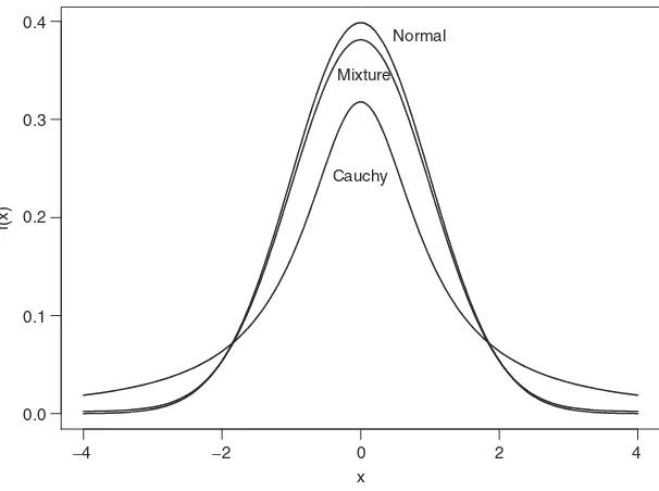
Figure 1.1. Comparison of finite mixture, stable, and standard normal density functions. Figure 1.1 shows the probability density functions of a finite mixture of normal, Cauchy, and standard normal random variable. The finite mixture of normal is (1₋X)N (0,1)₊X_×N (0,16) with X being Bernoulli such that P (X₌1)₌ 0.05, and the density function of Cauchy is

f (x)₌ 1

π(1₊x2₎, −∞< x <∞.

It is seen that the Cauchy distribution has fatter tails than the ﬁnite mixture of normal, which, in turn, has fatter tails than the standard normal.

1.2.3 Multivariate Returns

Let rt =(r1t, . . . , rNt)′ be the log returns of N assets at time t. The multivariate

analyses of Chapters 8 and 10 are concerned with the joint distribution of _{rt}T_t=1. This joint distribution can be partitioned in the same way as that of Eq. (1.15). The analysis is then focused on the speciﬁcation of the conditional distribution function F (rt|rt−1, . . . ,r1,θ). In particular, how the conditional expectation and conditional covariance matrix ofrt evolve over time constitute the main subjects of Chapters 8 and 10.

The mean vector and covariance matrix of a random vectorX₌(X1, . . . , Xp) are deﬁned as

(42)

provided that the expectations involved exist. When the data _{x1, . . . ,xT}of X are available, the sample mean and covariance matrix are deﬁned as

µ_x ₌ 1

T T

t=1

xt, x = 1 T ₋1

T

t=1

(xt−µx)(xt−µx)′.

These sample statistics are consistent estimates of their theoretical counterparts provided that the covariance matrix ofX exists. In the ﬁnance literature, the mul-tivariate normal distribution is often used for the log returnrt.

1.2.4 Likelihood Function of Returns

The partition of Eq. (1.15) can be used to obtain the likelihood function of the log returns _{r1, . . . , rT}of an asset, where for ease in notation the subscript i is omitted from the log return. If the conditional distribution f (rt|rt−1, . . . , r1,θ)is normal with meanµt and varianceσt2, thenθ consists of the parameters inµt and σ_t2 and the likelihood function of the data is

f (r1, . . . , rT;θ)=f (r1;θ) T

t=2 1

√

2π σt exp

−(rt−µt)2

2σ_t2 , (1.18)

wheref (r1;θ)is the marginal density function of the ﬁrst observationr1. The value of θ that maximizes this likelihood function is the maximum likelihood estimate (MLE) of θ. Since the log function is monotone, the MLE can be obtained by maximizing the log likelihood function,

lnf (r1, . . . , rT;θ)=lnf (r1;θ)− 1 2

T

t=2

ln(2π )₊ln(σ_t2)₊(rt−µt) 2

σ_t2 , which is easier to handle in practice. The log likelihood function of the data can be obtained in a similar manner if the conditional distributionf (rt|rt−1, . . . , r1;θ) is not normal.

1.2.5 Empirical Properties of Returns

(43)

s-rtn

−0.2 0.0 0.2

year

log-rtn

1940 1960 1980 2000

year

1940 1960 1980 2000

−0.3

−0.1 0.1 0.3

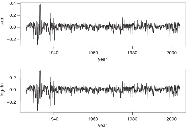
Figure 1.2. Time plots of monthly returns of IBM stock from January 1926 to December 2003. The upper panel is for simple returns, and the lower panel is for log returns.

year

s-rtn

1940 1960 1980 2000

year

1940 1960 1980 2000

−0.2 0.0 0.2 0.4

log-rtn

−_0.2

0.0 0.2

(44)

Table 1.2 provides some descriptive statistics of simple and log returns for selected U.S. market indexes and individual stocks. The returns are for daily and monthly sample intervals and are in percentages. The data spans and sample sizes are also given in the table. From the table, we make the following observations. (a) Daily returns of the market indexes and individual stocks tend to have high excess kurtosis. For monthly series, the returns of market indexes have higher excess kurtosis than individual stocks. (b) The mean of a daily return series is close to zero, whereas that of a monthly return series is slightly larger. (c) Monthly returns have higher standard deviations than daily returns. (d) Among the daily returns, market indexes have smaller standard deviations than individual stocks. This is in agreement with common sense. (e) The skewness is not a serious prob-lem for both daily and monthly returns. (f) The descriptive statistics show that the difference between simple and log returns is not substantial.

Figure 1.4 shows the empirical density functions of monthly simple and log returns of IBM stock. Also shown, by a dashed line, in each graph is the nor-mal probability density function evaluated by using the sample mean and standard deviation of IBM returns given in Table 1.2. The plots indicate that the normality assumption is questionable for monthly IBM stock returns. The empirical den-sity function has a higher peak around its mean, but fatter tails than that of the corresponding normal distribution. In other words, the empirical density function is taller and skinnier, but with a wider support than the corresponding normal density.

simple return

density

0.0

−40 −20 0 20 40 −40 −20 0 20 40

0.01 0.02 0.03 0.04 0.05 0.06

density

0.0 0.01 0.02 0.03 0.04 0.05 0.06

log return

(45)

1.3 PROCESSES CONSIDERED

Besides the return series, we also consider the volatility process and the behavior of extreme returns of an asset. The volatility process is concerned with the evolution of conditional variance of the return over time. This is a topic of interest because, as shown in Figures 1.2 and 1.3, the variabilities of returns vary over time and appear in clusters. In application, volatility plays an important role in pricing options and risk management. By extremes of a return series, we mean the large positive or negative returns. Table 1.2 shows that the minimum and maximum of a return series can be substantial. The negative extreme returns are important in risk management, whereas positive extreme returns are critical to holding a short position. We study properties and applications of extreme returns, such as the frequency of occurrence, the size of an extreme, and the impacts of economic variables on the extremes, in Chapter 7.

Other ﬁnancial time series considered in the book include interest rates, exchange rates, bond yields, and quarterly earning per share of a company. Figure 1.5 shows the time plots of two U.S. monthly interest rates. They are the 10-year and 1-year Treasury constant maturity rates from April 1954 to March 2004. As expected, the two interest rates moved in unison, but the 1-year rates appear to be more volatile. Figure 1.6 shows the daily exchange rate between the U.S. dollar and

rate

(a)

year

rate

1960 1970 1980 1990 2000

year

1960 1970 1980 1990 2000

(b) 15

10

5

0

15

10

5

0

(46)

PROCESSES CONSIDERED 21

Yens

(a)

(b)

year

Change

2000 2001 2002 2003 2004

year

2000 2001 2002 2003 2004

130

120

110

2 1 0

−1

−2

−3

−4

Figure 1.6. Time plot of daily exchange rate between U.S. dollar and Japanese yen from January 3, 2000 to March 26, 2004: (a) exchange rate and (b) changes in exchange rate.

the Japanese yen from January 2000 to March 2004. From the plot, the exchange rate encountered occasional big changes in the sampling period. Table 1.3 provides some descriptive statistics for selected U.S. ﬁnancial time series. The monthly bond returns obtained from CRSP are Fama bond portfolio returns from January 1952 to December 2003. The interest rates are obtained from the Federal Reserve Bank of St. Louis. The weekly 3-month Treasury bill rate started on January 8, 1954, and the 6-month rate started on December 12, 1958. Both series ended on April 9, 2004. For the interest rate series, the sample means are proportional to the time to maturity, but the sample standard deviations are inversely proportional to the time to maturity. For the bond returns, the sample standard deviations are positively related to the time to maturity, whereas the sample means remain stable for all maturities. Most of the series considered have positive excess kurtosis.

(47)

Table 1.3. Descriptive Statistics of Selected U.S. Financial Time Seriesa

Standard Excess

Maturity Mean Deviation Skewness Kurtosis Minimum Maximum

Monthly Bond Returns: January 1952 to December 2003,T =624

1–12 months 0.47 0.36 2.43 12.67 −0.40 3.52

24–36 months 0.53 0.99 1.40 12.93 −4.90 9.33

48–60 months 0.53 1.42 0.62 4.97 −5.78 10.06

61–120 months 0.55 1.71 0.63 4.86 −7.35 10.92

Monthly Treasury Rates: April 1953 to March 2004,T =612

1 year 5.80 3.01 0.96 1.27 −0.82 16.72

3 years 6.21 2.86 0.89 0.81 −1.47 16.22

5 years 6.41 2.79 0.88 0.67 −1.85 15.93

10 years 6.60 2.73 0.83 0.42 −2.29 15.32

Weekly Treasury Bill Rates: End on February 16, 2001

3 months 5.51 2.76 1.14 1.88 −0.58 16.76

6 months 6.08 2.56 1.26 1.82 −2.35 15.76

a_{The data are in percentages. The weekly 3-month Treasury bill rate started from January 8, 1954 and} the 6-month rate started from December 12, 1958. Data sources are given in the text.

EXERCISES

1.1. Consider the daily stock returns of American Express (axp), Caterpillar (cat), and Starbucks (sbux) from January 1994 to December 2003. The data are simple returns given in the ﬁled-3stock.txt (date, axp, cat, sbux). (a) Express the simple returns in percentages. Compute the sample mean, standard deviation, skewness, excess kurtosis, minimum, and maximum of the percentage simple returns.

(b) Transform the simple returns to log returns.

(c) Express the log returns in percentages. Compute the sample mean, stan-dard deviation, skewness, excess kurtosis, minimum, and maximum of the percentage log returns.

(d) Test the null hypothesis that the mean of the log returns of each stock is zero. (Perform three separate tests.) Use 5% signiﬁcance level to draw your conclusion.

(48)

REFERENCES 23

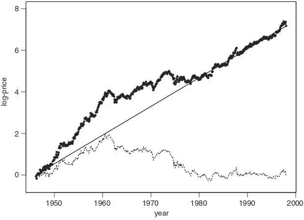
1.3. Consider the monthly stock returns of S&P composite index from January 1975 to December 2003 in Exercise 1.2. Answer the following questions: (a) What is the average annual log return over the data span?

(b) Assume that there were no transaction costs. If one invested $1.00 on the S&P composite index at the beginning of 1975, what was the value of the investment at the end of 2003?

1.4. Consider the daily log returns of American Express stock from January 1994 to December 2003 as in Exercise 1.1. Use the 5% signiﬁcance level to perform the following tests. (a) Test the null hypothesis that the skewness measure of the returns is zero. (b) Test the null hypothesis that the excess kurtosis of the returns is zero.

1.5. Daily foreign exchange rates (spot rates) can be obtained from the Federal Reserve Bank in Chicago. The data are the noon buying rates in New York City certiﬁed by the Federal Reserve Bank of New York. Consider the exchange rates between the U.S. dollar and the Canadian dollar, euro, U.K. pound, and Japanese yen from January 2000 to March 2004. (a) Compute the daily log return of each exchange rate. (b) Compute the sample mean, standard devia-tion, skewness, excess kurtosis, minimum, and maximum of the log returns of each exchange rate. (c) Discuss the empirical characteristics of the log returns of exchange rates.

REFERENCES

Campbell, J. Y., Lo, A. W., and MacKinlay, A. C. (1997).The Econometrics of Financial

Markets. Princeton University Press, Princeton, NJ.

Jarque, C. M. and Bera, A. K. (1987). A test of normality of observations and regression

residuals.International Statistical Review 55: 163–172.

Sharpe, W. (1964). Capital asset prices: A theory of market equilibrium under conditions of

risk.Journal of Finance19: 425–442.

Snedecor, G. W. and Cochran, W. G. (1980). Statistical Methods, 7th edition. Iowa State

(49)

Linear Time Series Analysis

and Its Applications

In this chapter, we discuss basic theories of linear time series analysis, introduce some simple econometric models useful for analyzing financial time series, and apply the models to asset returns. Discussions of the concepts are brief with empha-sis on those relevant to financial applications. Understanding the simple time series models introduced here will go a long way to better appreciate the more sophis-ticated financial econometric models of the later chapters. There are many time series textbooks available. For basic concepts of linear time series analysis, see Box, Jenkins, and Reinsel (1994, Chapters 2 and 3) and Brockwell and Davis (1996, Chapters 1–3).

Treating an asset return (e.g., log returnrt of a stock) as a collection of random variables over time, we have a time series{rt}. Linear time series analysis provides a natural framework to study the dynamic structure of such a series. The theories of linear time series discussed include stationarity, dynamic dependence, autocor-relation function, modeling, and forecasting. The econometric models introduced include (a) simple autoregressive (AR) models, (b) simple moving-average (MA) models, (c) mixed autoregressive moving-average (ARMA) models, (d) seasonal models, (e) unit-root nonstationarity, (f) regression models with time series errors, and (g) fractionally differenced models for long-range dependence. For an asset returnrt, simple models attempt to capture the linear relationship betweenrt and information available prior to time t. The information may contain the historical values ofrtand the random vectorYin Eq. (1.14) that describes the economic envi-ronment under which the asset price is determined. As such, correlation plays an important role in understanding these models. In particular, correlations between the variable of interest and its past values become the focus of linear time series anal-ysis. These correlations are referred to as serial correlationsor autocorrelations. They are the basic tool for studying a stationary time series.

Analysis of Financial Time Series, Second Edition By Ruey S. Tsay Copyright_{2005 John Wiley & Sons, Inc.}