Published by McGraw-Hill, a business unit of The McGraw-Hill Companies, Inc., 1221 Avenue of the Americas, New York, NY 10020. The first objective of the book is to develop those parts of the theory that are prominent in applications of the subject.
COMPLEX NUMBERS
SUMS AND PRODUCTS
Note that the right-hand sides of these equations can be obtained by formally manipulating the expressions on the left as if they involved only real numbers and replacing i2 with −1 when it occurs.
BASIC ALGEBRAIC PROPERTIES
1 The additive identity 0=(0,0) and the multiplicative identity 1=(1,0) for real numbers are transferred to the entire complex number system. Usei=(0,1)andy=(y,0)to verify that−(iy)=(−i)y. So show that the additive inverse of a complex number z=x+iy can be written −z = −x−iy without ambiguity.
FURTHER PROPERTIES
Prove that multiplication of complex numbers is commutative, as mentioned at the beginning of Sec. a) the associative law for adding complex numbers, mentioned at the beginning of Sec. Use the associative law of addition and the distributive law to show that z(z1+z2+z3)=zz1+zz2+zz3.
VECTORS AND MODULI
The geometric number is |z| is the distance between the point (x, y) and the origin, or the length of the radius vector representing z. 3, as it is only a statement that the length of one side of the triangle is less than or equal to the sum of the lengths of the other two sides.
COMPLEX CONJUGATES
The identity (7) is particularly useful in deriving the moduli properties from the conjugation properties mentioned above. By factoring z4−4z2+3 into two quadratic factors and using inequality (8), Sec. b) z is either real or pure imaginary if and only ifz2=z2.
EXPONENTIAL FORM
It should be emphasized that due to the constraint −π < ≤π of the main argument, it is not true that Arg(−1−i)=5π/4. MULTIPLICATIONS AND POWERS IN EXPONENTIAL FORMS Simple trigonometry tells us that eiθ has the familiar additive property expo-.
PRODUCTS AND POWERS IN EXPONENTIAL FORM Simple trigonometry tells us that e iθ has the familiar additive property of the expo-
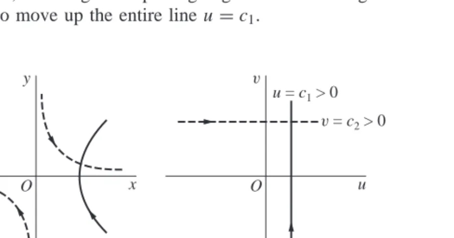
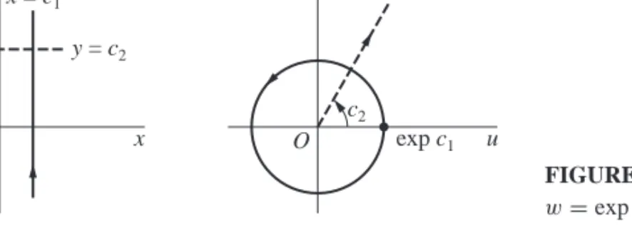
As the parameter θ increases from θ =0 to θ =2π, the pointer starts from the positive real axis and traverses the circle once counterclockwise. In general, the circle |z−z0| =R, whose center is z0 and whose radius is R, has the parametric representation.
Using the fact that the modulus|eiθ−1|is the distance between the pointveiθ and 1 (see Section 4), give a geometric argument to find a value of θ in the interval 0≤θ <2π that satisfies the equation|eiθ− 1| =2. By writing the individual factors on the left in exponential form, performing the necessary operations, and finally converting to rectangular coordinates, show that.
ROOTS OF COMPLEX NUMBERS
7 for integral powers of complex numbers z=reiθ, is useful in finding the nth roots of any non-zero complex number z0=r0eiθ0, where n has one of the values n=2,3,. From this exponential form of the roots, we can immediately see that they all lie on the circle|z| =√n.
EXAMPLES
When n≥3, the regular polygon on whose vertices the roots lie is inscribed in the unit circle |z| =1, where one vertex corresponds to the main root z=1(k=0). In view of expression (3), Sec. 9, the three cube roots of a non-zero complex number z0 can be written as c0, c0ω3, c0ω23, where c0 is the principal cube root of z0and.
REGIONS IN THE COMPLEX PLANE
It follows that if a set S is closed, then it contains each of its accumulation points. Thus a set is closed if and only if it contains all its accumulation points.
ANALYTIC FUNCTIONS
FUNCTIONS OF A COMPLEX VARIABLE
A generalization of the concept of function is a rule that assigns more than one value to a point z in the definition domain. When studying multivalued functions, one usually systematically assigns only one of the possible values assigned to each point, and constructs a (single-valued) function based on the multivalued function.
MAPPINGS
Then, since the image of a point (x,0) is (x2,0), that image moves to the right of the origin along the axis as (x,0) moves to the right of the origin along the axis. The image of the upper branch of the hyperbolax=1 is, of course, the horizontal line=2.
MAPPINGS BY THE EXPONENTIAL FUNCTION
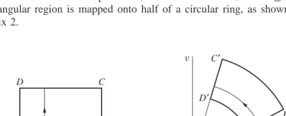
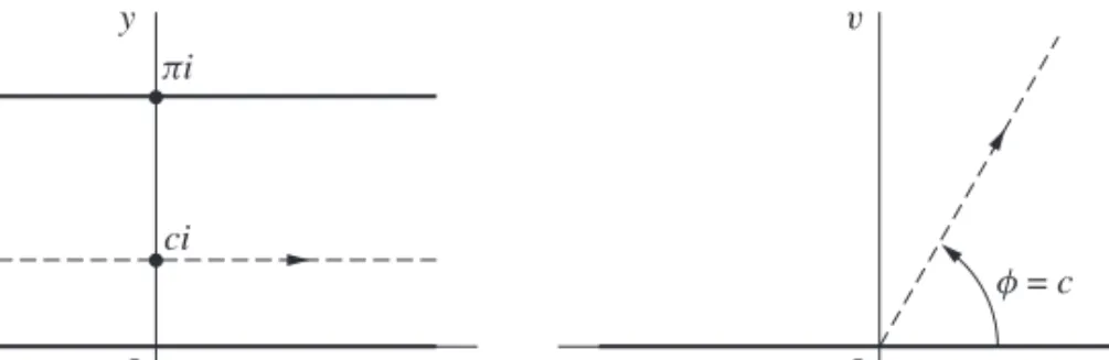
When w=ez, the image of the infinite strip 0≤y≤π is the upper half v≥0 of the w plane (Fig. 22). By considering the images of horizontal line segments, verify that the image of the rectangular region a≤x≤b, c≤y≤d under the transformation w=expz is the region ea≤ρ≤eb, c≤φ≤d, as shown in Fig.
LIMITS
An interpretation of a function w=f (z)=u(x, y)+iv(x, y) is that of a vector field in the domain of definition off. Condition (2) is thus satisfied by points in the range|z|<1 when δ is equal to 2ε or any smaller positive number.
THEOREMS ON LIMITS
This important theorem can be proved directly using the definition of the limit of a function of a complex variable. But, with the help of Theorem 1, it follows almost immediately from the theorems on the limits of real-valued functions of two real variables.
LIMITS INVOLVING THE POINT AT INFINITY
We begin the proof by noting that the first of the limits (1) means that for every positive number ε there exists a positive number δ, such that. The first of the limits (2) means that for every positive number ε there exists a positive number δ, such that.
CONTINUITY
16, that the function (5) is continuous at the point z0=(x0, y0) if and only if its components are continuous functions there. Show that S is unbounded (Section 11) if and only if every neighborhood of a point at infinity contains at least one point in S.
DERIVATIVES
When we take form (2) of the definition of the derivative, we often drop the subscript onz0 and introduce the number. However, it is true that the existence of the derivative of a function at a point implies the continuity of the function at that point. To see this, we assume that f(z0) exists and write
DIFFERENTIATION FORMULAS
It is thus legitimate to replace the variable w in equation (9) with f (z) when zi is any point in the neighborhood|z−z0|< δ. So equation (10) becomes equation (6) in the limit aszanapproachesz0. 19, of derived to give a direct proof that dw. 19, of derived to show that.
CAUCHY–RIEMANN EQUATIONS
Then the first-order partial derivatives of uandv must exist at (x0, y0), and they must satisfy the Cauchy–Riemann equations. Since the Cauchy–Riemann equations are necessary conditions for the existence of the derivative of a function f at a pointz0, it can often be used to locate points where f does not have a derivative.
The assumption that the first-order partial derivatives of u and v are continuous at the point (x0, y0) makes it possible to write∗. Sinceux=vyanduy = −vxeverywhere and since these derivatives are continuous everywhere, the conditions in the above statement are satisfied at all points in the complex plane.
POLAR COORDINATES
If the partial derivatives of u and v with respect to x and y also satisfy the Cauchy-Riemann equations. 23, from the Cauchy-Riemann equations, derives the alternative form. uθ+ivθ) of the expression forf(z0) from Exercise 8.
ANALYTIC FUNCTIONS
The chain rule for the derivative of a composite function shows that a composition of two analytic functions is analytic. More precisely, suppose that a function f (z) is analytic in a domain D and that the image (chapter 13) of D under the transformation w=f (z) is contained in the domain of the definition of a function g(w) .
EXAMPLES
As in example 3, we consider a function f that is analytic in a given domain D. Assuming that the modulus|f (z)|is constant through D, one can prove that f (z) must also be constant there. Then show that the composite function G(z)=g(z2+1) is analytic in the quadrant x >0, y >0, with the derivative.
HARMONIC FUNCTIONS
If two given functions are harmonic in a domain D and their first-order partial derivatives satisfy the Cauchy-Riemann equations (2) throughout D, v is said to be a harmonic conjugate of afu. 9 (Sec. 104) we shall show that a function u which is harmonic in a domain of a certain type always has a harmonic conjugate.
UNIQUELY DETERMINED ANALYTIC FUNCTIONS We conclude this chapter with two sections dealing with how the values of an ana-
Now suppose that two functions f and g are analytic in the same domain D and that f (z)=g(z) at every point z of some domain or line segment contained in D. A function that is analytic in a domain D is uniquely determined by its values in a domain, or along a line segment, contained in D.
REFLECTION PRINCIPLE
The function F is the analytic continuation in D1∪D2 of anyf1orf2; andf1 andf2 are called offF elements. Show that if the condition that f (x) is real in the reflection principle (Sec. 28) is replaced by the condition that f (x) is pure imaginary, then equation (1) in the statement of the principle is changed to .
ELEMENTARY FUNCTIONS
THE EXPONENTIAL FUNCTION
This is shown in the next section, where the logarithmic function is developed, and is illustrated in the following example. Then use the result in part (a), together with the property 1/ez=e−z(Sec. 29) of the exponential function.
THE LOGARITHMIC FUNCTION
3 It should be emphasized that it is not true that the left side of equation (3) reduces to justz by reversing the order of the exponential and logarithmic functions.
BRANCHES AND DERIVATIVES OF LOGARITHMS
The origin and radius θ =α constitute the branch cut for branch (2) of the logarithmic function. Find all the roots of the equation logz=iπ/2. a) functional (z)=Log(z−i) is analytic everywhere except for the part x≤0 of the line=1;.
SOME IDENTITIES INVOLVING LOGARITHMS
This means that the expression on the right here has different values, and those values are the roots of z. Thus show that log(z1/n)=(1/n)logzwhere corresponds to the value of log(z1/n) taken on the left, the corresponding value of logzis is chosen on the right and vice versa.
COMPLEX EXPONENTS
Note that although ez generally has a multiple value according to definition (10), the usual interpretation of ez occurs when the principal value of the logarithm is taken. Prove that if z=0 and is a real number, then|for| =exp(aln|z|)= |z|a, where the main value of|z|a should be taken.
TRIGONOMETRIC FUNCTIONS Euler’s formula (Sec. 6) tells us that
These functions are entire since they are linear combinations (Problem 3, Sec. 25) of the entire functionsseiz ande−iz. Knowing the derivatives. Note that the quotients tanz and secz are analytic everywhere except at the singularities (Sec. 24).
HYPERBOLIC FUNCTIONS
Find all the roots of the equation sinz=cosh 4 by equating the real parts and then the imaginary parts of sinzand cosh 4. 3 Because of the way in which the exponential function appears in definitions (1) and in definitions (Sec. 34) .
INVERSE TRIGONOMETRIC AND HYPERBOLIC FUNCTIONS
When specific branches of the square root and logarithmic functions are used, all three inverse functions will. Derivatives of the first two depend on the values chosen for the square roots:
INTEGRALS
CONTOURS
Derive the equation of the line through the points (α, a) and (β, b) in the plane τ shown in the figure. Let (x) be a real-valued function defined on the interval 0≤x≤1 by means of equations. b) Verify that arc C in part (a) is indeed a smooth arc.
CONTOUR INTEGRALS
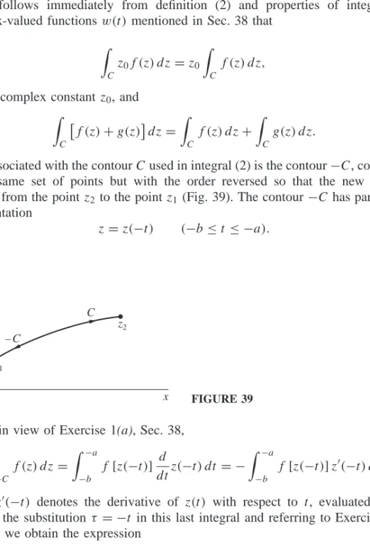
It immediately follows from the definition (2) and properties of integrals of functions with complex valuesw(t) mentioned in Sec. Except in special cases, no corresponding useful interpretation, geometric or physical, is available for integrals in the complex plane.
SOME EXAMPLES
Since the value of this integral depends only on the endpoints of C and is otherwise independent of the arc taken, we can write It follows from expression (6) that the integral of the function f (z)=za around each closed contour in the plane has the value zero. (Once again, compare with Example 2, where the value of the integral of a given function around a closed contour was not zero.) The question of predicting when an integral around a closed contour has the value zero will be discussed in Secs.
EXAMPLES WITH BRANCH CUTS
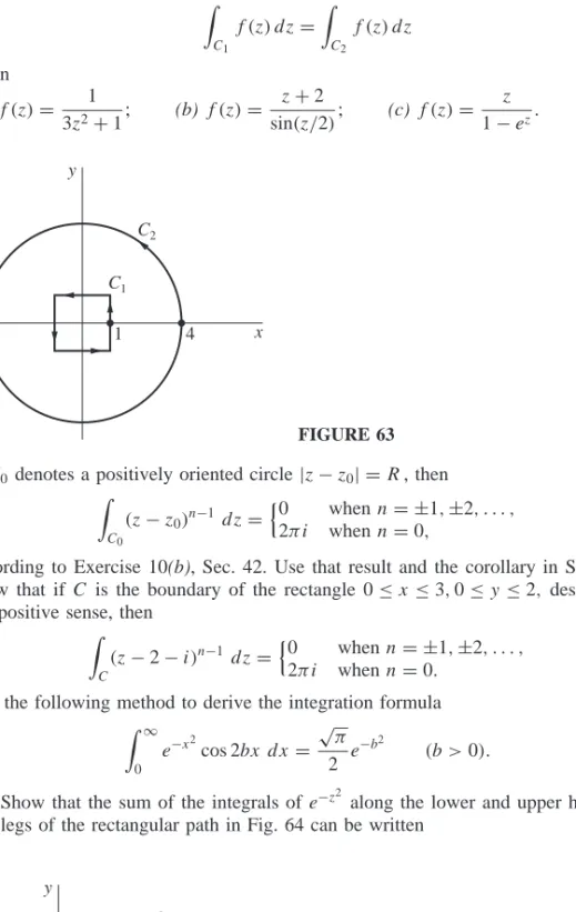
With the help of the result in exercise 3, Sec. command whole numbers and Cis the unit circle|z| =1, taken counterclockwise. Thus show that the value of the integral off (z)alongC is the same when the representation=Z(τ ) (α≤τ≤β) is used, instead of the original one.
UPPER BOUNDS FOR MODULI OF CONTOUR INTEGRALS
Then, dividing the numerator and denominator on the right here by R4, you show that the value of the integral tends to zero as R tends to infinity. Thus show that there is a positive constant A, independent of N, such that|sinz| ≥A for all points lying on the contour CN.
ANTIDERIVATIVES
The function f (z)=1/z2, which is continuous everywhere except at the origin, has an antiderivative F (z)= -1/z in the domain |z|>0, consisting of the entire plane with the origin deleted. . Note that the integral of the function (z)=1/cube around the same circle cannot be similarly evaluated.
PROOF OF THE THEOREM
To see that statement (b) implies statement (c), we now show that the value of any integral around a closed contour inD is zero when the integration is independent of the path there. Note that the value of the integral of function (5) around the closed contour C2−C1 in that example is, therefore,−4√.
CAUCHY–GOURSAT THEOREM
This is because the compound functionf (z)=exp(z3) is everywhere analytic and its derivativef(z)=3z2exp(z3) is everywhere continuous. If a function f is analytic at all points inside and on a simple closed contour C, then.
PROOF OF THE THEOREM
Given an arbitrary positive number ε, we consider the coverage of R in the statement of the lemma. As for the path lengthCj, it is 4sj if Cj is the boundary of a square.
SIMPLY CONNECTED DOMAINS
Since the value of the integral around each Ck is zero, it follows by the Cauchy–Goursat theorem. For a proof of the theorem involving more general paths of finite length, see, for example, Secs.
MULTIPLY CONNECTED DOMAINS
Show that if C is a positively oriented simple closed contour, the area of the region enclosed by C can be written. Prove that there exists a pointx0 that belongs to each of the closed intervalssan≤x≤bn.
CAUCHY INTEGRAL FORMULA Another fundamental result will now be established
Let the radius ρ of the circle Cρ be less than the number δ in the second of these inequalities. Because |z−z0| =ρ < δ when z is on Cρ, it follows that the first of inequalities (5) holds when z is such a point; and the theorem in Sec.
AN EXTENSION OF THE CAUCHY INTEGRAL FORMULA
To verify that f(z) exists and that expression (2) is in fact valid, we ledd note the smallest distance from the points, and use expression (1) to write. Letting z tend to zero, we find from this inequality that the right-hand side of equation (3) also tends to zero.
SOME CONSEQUENCES OF THE EXTENSION
Then write this integral in terms of θ to derive the integration formula π. a) Show using the binomial formula (Sec. 3) that the function for each value of n Hint: Use Cauchy's inequality (Sec. 52) to show that the second derivative f(z) is zero everywhere in the plane.
LIOUVILLE’S THEOREM AND THE FUNDAMENTAL THEOREM OF ALGEBRA
51, for the then derivative of the function, show that the polynomials in part (a) can be expressed in the form Butf is continuous in this closed disk, which means that f is also bounded there (Section 18).
MAXIMUM MODULUS PRINCIPLE
Suppose that a function f is continuous on a closed bounded region R and that it is analytic and not constant in the interior of R. Prove that the component functionu(x, y) has a minimum value inR, which occurs on the boundary of Rand and never inland.
SERIES
CONVERGENCE OF SEQUENCES An infinite sequence
Note that the value of n0 required will generally depend on the value of ε. Conversely, if we start with condition (4), we know that for every positive numberε there exists a positive integer.
CONVERGENCE OF SERIES An infinite series
Furthermore, we know from calculus that the nth term of a convergent series of real numbers approaches zero and tends to infinity. Furthermore, since the absolute convergence of the set of real numbers implies the convergence of the set itself, it follows that the set (8) both converge.