PRINCIPLES AND APPLICATIONS OF MICROEARTHQUAKE
NETWORKS
W. H . K . Lee and S . W. Stewart
OFFICE OF EARTHQUAKE STUDIES U. S. GEOLOGICAL SURVEY MENLO PARK. CALIFORNIA
1981
ACADEMIC PRESS
New York A Siibsidiary London Toronto Sydney San Francisco of Hurcoiirt Rrrrte Jovunm~ich. Piiblishers
COI’YRIGHI @ 1981, BY ACADLMIC PRESS, INC.
ALL RIGHTS RESERVED.
NO PART OF THIS PUBLICATION MAY BE REPRODUCED OR TRANSMITTED IN ANY FORM OR BY ANY MEANS, ELECTRONIC OR MECHANICAL, INCLUDING PHOTOCOPY, RECORDING, OR ANY INFORMATION STORAGE AND RE I RlEVAL SYSTEM, WITHOUT PERMISSION IN WRITING FROM THE PUBLISHER.
ACADEMIC PRESS, INC.
I l l Fifth Avenue. Ncw York. New York 10003
U I I I ‘ I P ~ K i f I ~ d O l 7 i Ediriorl prrblislred by
ACADEMIC PRESS, INC. (LONDON) LTD.
24/28 Oval Road, London N W I 7DX
LIBRARY OF CONGRESS CATALOG CARD NUMBER: 65-26406 ISBN 0-12-018862-7
PRINTED IN THE UNITED STATES OF AMERICA 81 82 83 84 9 8 7 6 5 4 3 2 1
Foreword
Earthquakes occur over a continuous energy spectrum, ranging from high-magnitude, but rare, earthquakes to those of relatively low mag- nitude but high frequency of occurrence (i.e., microearthquakes). This review is concerned primarily with the underlying physical principles, techniques, and methods of analysis used in studying the low-magnitude end of the spectrum. As a consequence of advancing technological capa- bilities that are being applied in many diverse regional networks, this subject has grown so rapidly that the need for a coherent overview de- scribing the present state of affairs seems clear.
One of the main reasons for the growth of interest in microearthquakes is a newly accepted concern of seismologists for prediction that goes along with the more traditional concerns for description and physical under- standing including the use of earthquake records as probes of internal constitution of the Earth. It is now recognized that these low-amplitude microearthquakes are important signals of continuous tectonic processes in the Earth, the future evolution of which is to be forecast. In this predic- tive respect seismology has moved closer in its goals to meteorology, inheriting the awesome difficulties of predicting the output of an essen- tially aperiodic, nonlinear, stochastic, dynamic system that can only be modeled and observed in a very crude way far short of the continuum requirements in space and time.
The observational difficulties in seismology are, in fact, even more acute than those in meteorology. As we have indicated, however, there have already been substantial advances in this aspect of the problem, and this Supplement 2 volume of Advcrnces iw Geophysics, by Lee and Stewart, will provide a benchmark for the progress made to date.
BARRY SALTZMAN
vii
Preface
In the fall of 1976, Professor Stewart W. Smith invited us to contribute an article on “Network Seismology as Applied to Earthquake Prediction”
for a volume in the Advances in Geophysics serial publication. We felt that a review of microearthquake networks and their applications would be more appropriate with respect to our experience. The manuscript grew in size beyond the usual length of a review article. We are grateful that Professor Barry Saltzman, the Editor of Advtrrzces in Geophysics, accepted the manuscript for publication as a supplemental volume in this series.
Seismology is the study of earthquakes and the Earth’s internal struc- ture using seismic waves generated by earthquakes and artificial sources.
Individual earthquakes vary greatly in the amounts of energy released. In 1935, C. F. Richter introduced the concept of earthquake magnitude-a single number that quantifies the “size” of an earthquake based on the logarithm of the maximum amplitude of the recorded ground motion.
Earthquakes of magnitude less than 3 usually are called microearth- quakes. They are felt over a relatively small area, if at all. The great earthquakes, those of magnitude 8 or larger, cause severe damage if they occur in populated areas. In 1941, B. Gutenberg and C. F. Richter discov- ered that the logarithm of the number of earthquakes in a given magnitude interval varies inversely with the magnitude. In general, the number of earthquakes increases tenfold for each decrease of one unit of magnitude.
Thus, microearthquakes of magnitude 1 are several million times more frequent than earthquakes of magnitude 8.
The principal tool in seismology is the seismograph, which detects, amplifies, and records seismic waves. Because the seismic energy re- leased by microearthquakes is small, seismographs with high amplifica- tion must be used. With the advances in electronics in the 1950s, sensitive seismographs were developed. Thus, it became practical by the 1960s to operate an array of closely spaced and highly sensitive seismographs to study the more numerous microearthquakes. Such an array is called a microearthquake network.
ix
Microearthquake networks are especially well suited for intensively studying seismically active areas and are a powerful tool for investigating the earthquake process in great detail and in relatively short time inter- vals. Their applications are numerous, such as monitoring seismicity for earthquake prediction purposes, mapping active faults for hazard evalua- tion, exploring for geothermal resources, and investigating the Earth’s crust and mantle structure.
As far as we are aware, this book is the first attempt to present a review of the fundamentals of microearthquake networks: instrumentation sys- tems, data processing procedures, methods of data analysis, and examples of applications. Because microearthquake networks have been developed by many independent groups in several countries, it is difficult for us to present a comprehensive review. Rather, we have relied heavily upon our experience with the USGS Central California Microearthquake Network.
In this book, we have emphasized methods and techniques used in mi- croearthquake networks. Results from applications of microearthquake networks are tabulated and referenced, but not described in any detail.
We believe that interested persons should read the original articles. Due to space and time limitations, we have not treated several relevant topics, such as the principles of seismometry, and some recently developed tech- niques in digital instrumentation and data analysis. However, some refer- ences to these and related topics are provided.
A considerable amount of practical material relevant to earthquake seismology has been brought together here. We believe that this volume will be useful especially to those who wish to operate a microearthquake network or to interpret data from it. Each chapter has been written to be reasonably self-contained. Two preparatory chapters on seismic ray trac- ing, generalized inversion, and nonlinear optimization are given so that basic techniques in microearthquake data analysis can be developed sys- tematically. In addition to author and subject indexes, a glossary of ab- breviations and unusual terms has been prepared to help the reader. This work is intended for seismologists in general, and for those geologists, geophysicists, and engineers who wish to learn more about micro- earthquake networks and their applications.
We thank many of our colleagues for sending us preprints and reprints of their work in microearthquake studies, and for answering questions. It is a pleasure to acknowledge suggestions and comments on the manuscript by K. Aki, D. J. Andrews, R. Archuleta, U. Ascher, W. H. Bakun, M.
Bath, B. A. Bolt, M. G. Bonilla, D. M. Boore, C. G. Bufe, R. Buland, P.
T. Burghardt, U. Casten, R. P. Comer, C. H. Cramer, S. Crampin, R.
Daniel, J. P. Eaton, N. Gould, T. C. Hanks, D. H. Harlow, T. L. Henyey, R. B. Herrmann, D. P. Hill, J. Holt, R. Jensen, J. C. Lahr, J. Langbein,
Prt-fiice xi J. Lawson, F. Luk, T. V. McEvilly, W. D. Mooney, S. T. Morrissey, R. D.
Nason, M. E. O'Neill, R. A. Page, N. Pavoni, R. Pelzing, V. Pereyra, L.
Peselnick, G. Poupinet, C. Prodehl, M. R. Raugh, P. A. Reasenberg, I.
Reid, A. Rite, J. C. Savage, R. B. Smith, P. Spudich, D. W. Steeples, C.
D. Stephens, Z. Suzuki, J. Taggart, P. Talwani, C. Thurber, R. F. Yerkes, and Z. H. Zhao.
We are grateful to I. Williams for typing the manuscript, to R. Buszka and R. Eis for drafting some of the figures, to W. Hall, W. Sanders, and J. Van Schaack for technical information, and to B. D. Brown, S. Caplan, K. Champneys, D. Hrabik, M. Kauffmann-Gunn, K. Meagher, A. Rapport, and J. York for assistance in preparing and proofreading the manuscript.
The responsibility for the content of this book rests solely with the authors. We welcome communications from readers, especially concern- ing errors that they have found. We plan to prepare a Corrigenda, which will be available later for those who are interested.
W. H. K. LEE
s.
w . STEWART1. Introduction
Earthquakes of magnitudes less than 3 are generally referred to as mi- croearthquakes. In order to extend seismological studies to the micro- earthquake range, it is necessary to have a network of closely spaced and highly sensitive seismographic stations. Such a network is usually called a microearthquake network. It may be operated by telemetering seismic signals to a central recording site or by recording at individual stations.
Depending on the application, a microearthquake network may consist of several stations to a few hundred stations and may cover an area of a few square kilometers to 1 0 km2. Microearthquake networks became opera- tive in the 1960s; today, there are about 100 permanent networks all over the world (see Section 7. I ) . These networks can generate large quantities of seismic data because of the high occurrence rate of microearthquakes and the large number of recording stations.
By probing in seismically active areas, microearthquake networks are powerful tools in studying the nature and state of tectonic processes.
Their applications are numerous: monitoring seismicity for earthquake prediction purposes, mapping active faults for hazard evaluation, explor- ing for geothermal resources, investigating the structure of the crust and upper mantle, to name a few. Microearthquake studies are an important component of seismological research. Results from these studies are usu- ally integrated with other field and theoretical investigations in order to understand the earthquake-generating process.
In the following sections, we present a brief historical account of the development of microearthquake studies and give an overview of the contents and scope of the present work.
1.1, Historical Development
Microearthquake studies were stimulated by the introduction of the earthquake magnitude scale by C. F. Richter in 1935, and by the discovery
2 1 . Introduction
of the earthquake frequency-magnitude relation by B. Gutenberg and C.
F. Richter in 1941 (a similar relation between maximum trace amplitude and frequency of earthquake occurrence was found by M. Ishimoto and K. Iida in 1939). Implementation of microearthquake networks in the 1960s was made possible by technological advances in instrumentation, data transmission, and data processing.
In order to implement a nuclear test ban treaty in the late 1950s, exten- sive seismological research in detecting nuclear explosions and in dis- criminating them from earthquakes at teleseismic distances was carried out with support from various governments. Several arrays of seismom- eters in specific geometrical patterns were deployed in the 1960s. The largest and best known of these is the Large Aperture Seismic Array (LASA) in Montana. It consisted of 21 subarrays, each with 25 short- period, vertical-component seismometers (arranged in a circular pattern) and a set of long-period, three-component seismometers at the subarray center (Capon, 1973). Four smaller arrays were sponsored by the United Kingdom Atomic Energy Authority (Corbishley, 1970): these were lo- cated at Eskdalemuir, Scotland (Truscott, 1964); Yellowknife, Canada (Weichert and Henger, 1976); Gauribidanur, India (Varghese et al., 1979);
and Warramunga, Australia (Cleary et al., 1968). Four smaller arrays were also established in Scandinavian countries: the NORSAR array in Nor- way (Bungum and Husebye, 1974), the Hagfors array in Sweden, and the Helsinki and Jyvaskyla arrays in Finland (Pirhonen et al., 1979).
Some of these arrays were among the first ever to combine digital computer methods for on-line event detection and off-line event process- ing. They pioneered the way for automating the processing of seismic data. However, these earlier seismic arrays were concerned almost exclu- sively with studying teleseismic events. It is beyond our scope to discuss them further.
In terms of historical development, microearthquake networks evolved from regional and local seismic networks rather than from seismic arrays for nuclear detection. Microearthquake networks also evolved from tem- porary expeditions that studied aftershocks of large earthquakes to recon- naissance surveys, and finally to permanent telemetered networks or highly mobile arrays of stations. Methods and techniques to study mi- croearthquakes have been developed (more or less independently) by vari- ous groups in several countries, notably in Japan, South Africa, the United States, and the USSR.
Although historical development of microearthquake studies in the countries mentioned above will be discussed in Sections 1 . 1 .&I. 1.7, many pioneering investigations have been carried out in other countries as well. For example, Quervain (1924) appeared to be the first to use a
1.1. Historical Development 3 portable seismograph to record aftershocks. By deploying an instrument near the epicenter of a strong local earthquake in Switzerland and by recording in Zurich also, he was able to use the aftershocks to estimate P and S velocities in the earth’s crust.
I .I . I . Magnitude Scale
Richter (1935) developed the local magnitude scale using data from the Southern California Seismic Network operated by the California Institute of Technology. At that time, this network consisted of about 10 stations spaced at distances of about 100 km. The principal equipment was the Wood-Anderson torsion seismograph (Anderson and Wood, 1925) of 2800 static magnification and 0.8 sec natural period. Richter defined the local magnitude of an earthquake at a station to be
( 1 . 1 )
where A is the maximum trace amplitude in millimeters recorded by the station’s Wood-Anderson seismograph, and the term -log A . is used to account for amplitude attenuation with epicentral distance. The concept of magnitude introduced by Richter was a turning point in seismology because it is important to be able to quantify the size of earthquakes on an instrumental basis. Furthermore, Richter’s magnitude scale is widely ac- cepted because of the simplicity in its computational procedure. Subse- quently, Gutenberg ( 1945a,b,c) generalized the magnitude concept to in- clude teleseismic events on a global scale.
Richter realized that the zero mark of the local magnitude scale is arbitrary. Since he did not wish to deal with negative magnitudes in the Southern California Seismic Network, he chose the term -log A. equal to 3 at an epicentral distance of 100 km. Hence earthquakes recorded by a Wood-Anderson seismograph network are defined to be mainly of mag- nitude greater than 3, because the smallest maximum amplitude readable is about 1 mm. In addition, the amplitude attenuation is such that the term -log A. equals 1.4 at zero epicentral distance. Therefore, the Wood- Anderson seismograph is capable of recording earthquakes to magnitude of about 2, provided that the earthquakes occur very near the station (Richter and Nordquist, 1948).
I .I .2. Frequency-Magnitude Relation
In the course of detailed analysis of earthquakes recorded in Tokyo, Ishimoto and Iida (1939) discovered that the maximum trace amplitude A of earthquakes at approximately equal focal distances is related to their
4 1. Iiitroduction frequency of occurrence N by
(1.2) NA‘” = k (const)
where m is found empirically to be 1.74. At about the same time, Guten- berg and Richter (1941) found that the magnitude M of earthquakes is related to their frequency of occurrence by
(1.3) log N = a - bM
where a and b are constants. The Ishimoto-Iida relation does not lead directly to the frequency-magnitude formula [Eq. (1.3)] because the max- imum trace amplitude recorded at a station depends on both the mag- nitude of the earthquake and its distance from the station. However, under general assumptions, the frequency-magnitude formula can be de- duced from the Ishimoto-Iida relation as shown by Suzuki (1953).
Many studies of earthquake statistics have shown that Eq. (1.3) holds and that the value of b is approximately 1. This means that the number of earthquakes increases tenfold for each decrease of one magnitude unit.
Therefore, the smaller the magnitude of earthquakes one can record, the greater the amount of seismic data one collects. Microearthquake net- works are designed to take advantage of this frequency-magnitude rela- tion.
I J . 3 .
Seismologists have used words such as “small” or “large” to describe earthquake size. After the introduction of Richter’s magnitude scale, it was convenient to classify earthquakes more definitely to avoid am- biguity. The usual classification of earthquakes according to magnitude is as follows (Hagiwara, 1964):
ClassiJication of Earthquakes by Magnitude
Magnitude ( M ) Classification M 2 7
5 5 M < 7 3 5 M < 5 1 5 M < 3
Major earthquake (“great” for M 2 8) Moderate earthquake
Small earthquake Microearthquake
M < I Ultra-microearthquake
There is now a tendency to denote as microearthquakes all earthquakes of magnitude less than 3, and the term ultra-microearthquake is seldom used. However, in the existing literature, terms like “small,” “very small,” “minimal,” “weak,” and “local” are often used to describe earthquakes of microearthquake size.
1 . 1 . Historicul Development S Because the dynamic range of seismic recordings is only of the order of lo2 - I@’. different seismic networks are designed to study earthquakes of different magnitude ranges. For example, the World-Wide Standardized Seismograph Network (Oliver and Murphy, 1971) is designed to study earthquakes of magnitude between 5.5 and 7.5; regional networks (such as the Southern California Seismic Network used by C. F. Richter to de- velop the local magnitude scale) are designed to study small and moderate earthquakes ( 3 5 M < 6); and microearthquake networks are designed to study micro- and ultra-microearthquakes ( M < 3). If an earthquake of magnitude larger than the designed magnitude range of a network oc- curred within the network, instrumental saturation would not allow a complete study of the seismograms, but the first P-arrival times and first P-motion readings would permit precise locations and fault-plane solu- tions of the earthquakes.
1 .I .4.
Earth tremors related to deep gold mining operations were first noticed in the Witwatersrand region of South Africa in 1908 (Gane rt al., 1946). In 1910 a 200-kg Wiechert horizontal seismograph was installed about 6.5 km north of the mining area. The records showed that many more tremors occurred than were felt. Later, it became apparent that the average tremor intensity and rate of occurrence were increasing, along with the rate of tonnage mined and the depth of mining.
In the late 1930s a group at the Bernard Price Institute of Geophysical Research began a detailed study of these tremors. Although the tremors were assumed to be related directly to the mining activity (an early exam- ple of man-made earthquakes), their exact location was the first question to be answered. In 1939 five mechanical seismographs were constructed and deployed in an array specifically to locate the tremors [Gane et ul.
(194611. They recognized that a frequency response up to 20 Hz and a timing resolution of 0.1 sec or better would be necessary. By establishing a seismic network for high-quality hypocenter determination, they showed that the tremors were indeed originating from within the mining area, and more specifically, from within those areas mined during the preceding 10 years.
More detailed studies of a larger number of tremors, with greater timing resolution, were needed. Gane et ul. (1949) described a six-station radiotelemetry seismic network that they designed and applied to this problem. At the central recording site there was a multichannel photo- graphic recorder with an automatic trigger to start recording when an earthquake was sensed. A 6-sec magnetic tape-loop delay line to preserve
Development in South Africa
6 1. Introduction
the initial P-onsets was devised. The early foresight of this research group in specifying the requirements of instrumental networks to study mi- croearthquakes and their ingenuity in the design, construction, and opera- tion of this particular network deserve to be recognized.
1 .I .5.
Because of frequent damaging earthquakes occurring in and near Japan, Japanese seismologists pioneered in many aspects of earthquake re- search. In order to observe earthquakes in epicentral areas, Japanese seismologists (notably A. Imamura and M. Ishimoto) developed portable seismographs to study aftershocks and to monitor seismicity. The works by Imamura (1929), Imamuraet al. (1932). Nasu (1929a,b, 1935a,b, 19361, Iida (1939, 1940). Omote (1944, 1950a,b, 1955), and many others greatly contributed to our knowledge of aftershocks. The paper that first intro- duced the word "microearthquake" was by Asada and Suzuki (1949).
They chose this word to be equivalent to the Japanese word bisho zisin.
which means very small or smaller than small earthquake (Z. Suzuki, written communication, 1979).
Asada (1957) reported the first detailed study of microearthquakes. He demonstrated that many microearthquakes could be detected in and near Kanto district by ultrasensitive seismographs having a magnification of lo7 at 20 Hz. Asada understood the technical requirements of recording microearthquakes and the advantages of studying microearthquakes be- cause of their higher rate of occurrence. He investigated the frequency- magnitude relationship for microearthquakes, and tried to determine whether microearthquakes also occur in seismic regions where larger earthquakes occur. He foresaw the potential of using microearthquakes to predict larger earthquakes.
Detailed studies of microearthquakes in the Kii Peninsula, central Japan, using temporary arrays of short-period instruments and radio- telemetry seismograph systems were carried out by Miyamura and his colleagues in the 1950s and early 1960s (1966, with references therein to earlier works). Timing accuracy was stressed in order to obtain precise locations for the microearthquakes. Miyamura ( 1960) achieved an accu- racy of k0.05 sec by using a recording paper speed of 4 m d s e c . Miyam- ura et al. (1964) also used triggered magnetic tape recorders with a small four-station array in Gifu Prefecture, central Japan. An endless tape loop with a 20-sec delay time allowed recording of the initial P-onsets. An automatic gain control system was used to allow better readings of the S-phases.
The well-known Matsushiro earthquake swarm was first observed at Development in Japan
1.1. Historical Development 7 the Matsushiro Seismological Observatory in August 1965. The swarm activity increased remarkably, with more than 6000 microearthquakes recorded daily by March 1966. By mid-April slightly more than 600 earthquakes were felt in one day (Rikitake, 1976). Many special studies, including seismic and geodetic observations, were conducted. The papers are too numerous to review here, but readers may consult, for example, the Bulletin of the Earthquake Research Institute, University of Tokyo.
In the 1960s many microearthquake networks were established in Ja- pan. These networks consisted of about 5-15 stations each and were operated by many groups (Suzuki et al., 1979). More recently, an effort was made to combine microearthquake data from several groups into a central data processing center (T. Usami, personal communication, 1979).
This should mark a new era in microearthquake studies in Japan.
1.1.6. Development in USSR
The study of microearthquakes in the Soviet Union was initiated by G.
A. Gamburtsev and his colleagues. The early history was documented by Riznichenko (1975). In the late 1940s Gamburtsev applied the experience gained in seismic prospecting to the study of local weak earthquakes (Soviet seismologists often used the term “weak” earthquakes to denote microearthquakes). In 1949 and 1953 Complex Seismological Expeditions were conducted in Turkmenia to map the focal region of the 1948 Ashkhabad earthquake. Networks of temporary stations were installed to make detailed studies of the seismicity (Rustanovich, 1957; Gamburtsev and Gal’perin, 1960a). In 1953 detailed studies of microearthquake dis- tribution were camed out in the epicentral region of the 1946 Khait earthquake in the Tadzhik Republic (Gamburtsev and Gal’perin, 1960b).
A major contribution by Gamburtsev was to organize the Tadzhik Joint Seismological Expedition in the Garm and Khait regions beginning in 1954. Gamburtsev and his colleagues realized that microearthquakes could provide large quantities of data to establish relations between mi- croearthquakes and large events and to obtain knowledge of the earthquake-generating process. The first stage of this expedition in 1955-
1957 resulted in the publication of the monograph Methods of Detailed Investigations of Seismicity edited by Riznichenko ( 1960).
I. L. Nersesov became head of the Tadzhik Joint Seismological Expedi- tion when Gamburtsev died in 1955. The expedition had a major role in the development of a new generation of seismologists in the USSR, and in the quantification of seismicity and seismic risk (Riznichenko, 1975). Nerse- sov and his colleagues at Garm generally are credited with providing a worldwide stimulus for earthquake prediction. In the 1960s they reported
8 1. Introduction
that changes in the travel time ratio t $ I , preceded earthquakes of moder- ate size (Kondratenko and Nersesov, 1962; Semenov, 1969).
Fedotov and his colleagues at the Institute of Volcanology, Petropavlovsk-Kamchatsky, USSR, made detailed studies of seismicity in the Kamchatka-Kuriles region. They developed the concept of seismic gaps and seismic cycles for the prediction of large earthquakes (Fedotov,
1965, 1968; Fedotov et d., 1969).
Telemetered microearthquake networks were developed only recently in the Soviet Union, in cooperation with American seismologists (Wallace and Sadovskiy, 1976).
1.1.7.
Systematic studies of local earthquakes in southern California began in the 1920s through the effort of H. 0. Wood. Anderson and Wood (1925) developed the Wood-Anderson seismograph, a remarkably simple and sensitive instrument at that time. From the 1920s to the 1950s Wood- Anderson seismographs formed the backbone of the Southern California Seismic Network, which was first operated by the Carnegie Institution of Washington and later by the California Institute of Technology. Similar studies of local earthquakes in northern California were carried out by the Seismographic Stations of the University of California. Even though mi- croearthquakes occurring near a station could be recorded, these regional networks were not adequate to investigate microearthquakes, because station spacing was sparse and instrument sensitivity was not high enough. The first reported microearthquake study in the United States was made by Sanford and Holmes (1962) near Socorro, New Mexico, in a manner similar to that used by Asada (1957).
In the 1950% J. P. Eaton developed a telemetered seismograph system (peak magnification of 40,000 at 5 Hz) for the Hawaii Seismic Network.
The stations were deployed densely enough to permit precise location of microearthquakes on a routine basis (Eaton, 1962). From 1961 to 1963, Don Tocher upgraded the Seismographic Stations of the University of California by telemetering seismic signals from individual stations via telephone lines to a central recording center at Berkeley (Bolt, 1977a).
Thus by the early 1960s the key elements for a telemetered seismic net- work were known.
At about the same time, portable seismographs of high sensitivity were also developed (e.g., Lehner and Press, 1966). Several groups in the United States began microearthquake surveys. Notable among these were J. Oliver and his colleagues at the Lamont-Doherty Geological Obser- vatory (e.g., Oliverer a / . , 19661, and J . N. Brune and his colleagues at the
Development in the United States
Caltech Seismological Laboratory (e.g., Brune and Allen, 1967). A de- tailed study of the aftershocks of the 1966 Parkfield earthquake by Eaton et (11. ( 1970b) demonstrated that microearthquakes were useful in delineat- ing the slip surface of the Parkfield earthquake in three dimensions. This experience led Eaton and his colleagues of the U.S. Geological Survey (USGS) to develop the Central California Microearthquake Network on a large scale (Eaton et al.. 1970a). Beginning with three local clusters of stations in 1967, this network has grown to include 250 stations covering central California in 1980.
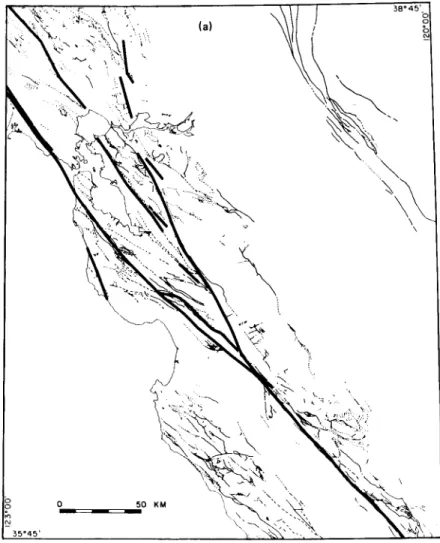
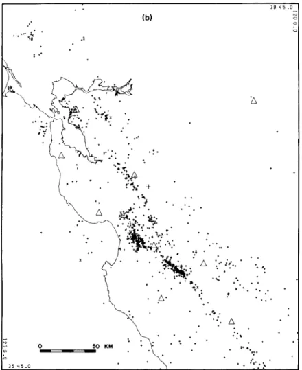
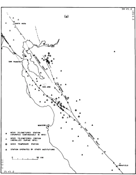
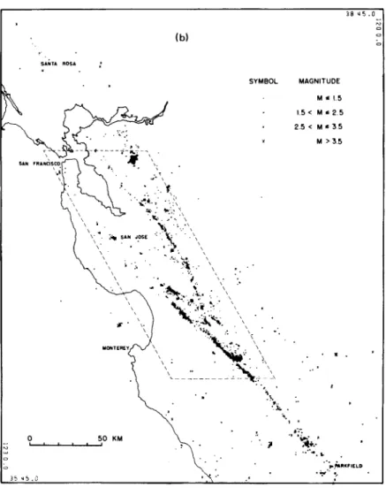
Figures I and 2 illustrate one of the capabilities of a dense microearth- quake network (such as the USGS Central California Microearthquake Network). Figure la shows numerous faults mapped in the network re- gion. Figure Ib shows earthquake epicenters determined by a good re- gional network operated by the Seismographic Stations of the University of California at Berkeley for a nine-year period. With a dense network of stations, as shown in Fig. 2a, the spatial distribution of earthquake epicen- ters delineates their relationship to active faults in only one year’s obser- vation, as shown in Fig. 2b.
In addition to several microearthquake networks developed and oper- ated by the U.S. Geological Survey, others have been implemented by various universities, for example, University of Washington (Crosson,
1972). St. Louis University (Stauder et
LII.,
1976), and the Lamont- Doherty Geological Observatory of Columbia University (Sykes, 1977).In the 1970s, various agencies of the United States government became concerned about earthquake hazards and supported the development and operation of many microearthquake networks. Today, about 50 perma- nent networks are operating in the United States (see Section 7. I).
Aggarwal rt cil. ( 1973) were the first to establish a network of portab!e seismographs in the United States specifically to search for precursory velocity anomalies similar to those reported from the Garm region, USSR.
They studied a swarm of microearthquakes in the Blue Mountain Lake area of New York State. Detailed analysis of V,/V, ratios showed the same type of behavior as in the Garm region, and changes preceding earthquakes as small as magnitude 2.5 and 3.3 were observed (Aggarwal et d., 1973, 1973. Using stations from the Southern California Seismic Network, Whitcomb e f 01. (1973) reported similar precursory behavior preceding the destructive San Fernando earthquake of February 9, 1971.
1.2. Overview and Scope
This work reviews some principles and applications of microearthquake networks. In summarizing the present status, we emphasize methods and
10 1. Introduction
Fig. la. Schematic map showing fault traces in central California. The heavy lines delineate major active faults.
techniques instead of results. Our review draws heavily on our experience with the Central California Microearthquake Network of the U.S. Geolog- ical Survey.
In Chapter 2 we describe mainly the instrumentation system employed in the USGS Central California Microearthquake Network. We emphasize the data processing systems of the same network in Chapter 3. Chapters 4 and 5 contain mathematical and computational preliminaries required in modern analyses of microearthquake data. Although numerous papers
1.2. Overview and Scope
t.
x
'n
3 8 4 5 .o
* * .**
*:. .
At .
I t 1 .
*
.'
0 - - I )50 KM
.
**. - 1Fig. Ib. Map showing earthquake epicenters (for the period 1962-1970) as determined by the Seismographic Stations of the University of California at Berkeley. Station sites are shown as triangles.
have been published on generalized inversion, nonlinear optimization, and seismic ray tracing, uniformly developed and readable accounts of these topics for seismologists seem to be lacking. Therefore, we attempt to present these topics in an introductory manner. Chapter 6 deals with methods of locating microearthquakes, of fault-plane solutions, and of magnitude estimation. Simultaneous inversion of hypocenter parameters and velocity structure is also discussed.
12 1. Ititroductioti
3 8 4 5 .o
b
A
A
A WCER TELEYETERED I T I l l O l l IOPLIATLO CONTINUOUSLY IN IS701 NCLR TELLYETERED SlAlION IINSTALLLD numa ISTO) 0 NCER T E Y f U l A R l S l A l t O N
0 so " Y
3 5 45.0
Fig. Za. Map showing seismographic stations in central California for 1970.
Chapters 7 and 8 review various applications of microearthquake net- works in earthquake prediction, hazard evaluation, exploration for geo- thermal energy, and studies of crustal and upper mantle structure. Chapter 9 is a brief summary of our personal views on microearthquake studies and a few comments on the future development of microearthquake networks.
We have tried to keep mathematical notation consistent within each chap- ter, but it may vary from one chapter to another. This is due in part to differences in notation between the mathematical and seismological litera- ture.
Fig. 2b. Map showing earthquake epicenters (for 1970) as determined by the USGS Central California Microearthquake Network using stations shown in part (a).
Microearthquake studies have been published in a wide variety of jour- nals and reports. They also appear in languages other than English, such as Japanese, Russian, Chinese, German, and French. In the course of preparing this work, we have collected more than 2000 articles related to this subject. It is clearly beyond our abilities to treat every article equally and fairly, especially the non-English papers. Nevertheless, we have se- lected about 700 papers and books for references. The reference list is arranged alphabetically by authors. If the paper is not in English, we have
14 1. Introduction
indicated the language in which it is written. We have cited many USGS Open-File Reports, which are on file at the libraries of the
U.S.
Geological Survey in Reston, Virginia; Denver, Colorado; and Menlo Park, Califor- nia.We hope that this work will provide some guidance for scientists begin- ning this field of research and will serve as a general reference on mi- croearthquake studies. In an attempt to make this book more useful to readers, we have prepared a Glossary, an Author Index, and a Subject Index. If a certain term is not familiar to the reader, the following steps are recommended: (1) consult the Subject Index and refer to the pages where the term in question may be defined or discussed, (2) consult the Glossary, or (3) consult the standard references given in the Glossary.
The Author Index lists all the names that appear explicitly in the text. A paper with three or more authors is referred to in the text by the name of the first author followed by et al. Because the names of the other authors in this case do not appear explicitly, they are not indexed. However, all authors in the References section are included in the Author Index.
2. Instrumentation Systems
2.1. General Considerations
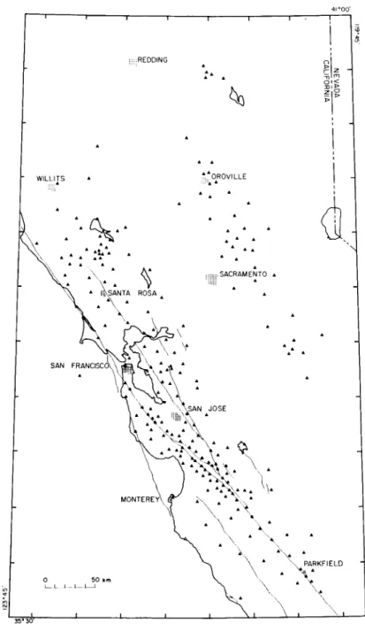
Some microearthquake networks are intended to study seismicity and active tectonic processes in relatively large regions. Others are set up for a single objective (e.g., to evaluate particular sites for emplacement of criti- cal structures such as dams or nuclear power plants). In a n y case, the expected function of a microearthquake network should be the primary concern in its design and operation. It is not our intent to discuss in detail the design principles of all types of microearthquake networks. Rather, we will review some factors that should be considered in laying out a microearthquake network. These include: the merits of a centralized re- cording, timing, and processing system; some considerations for station location; and an approach to the selection of an optimal frequency re- sponse for the system. In all cases we assume that the first function of a network is to locate earthquakes that occur within the network and to compute their magnitudes. We and our colleagues in Menlo Park have been developing the large USGS network in central California (Fig. 3) for many years. We will describe our techniques in some detail because many of them could be applied to other networks. Finally, we will briefly sum- marize some features of other microearthquake networks.
2.1 . I . Centralized Recording Systems
Telemetry transmission and centralized timing and recording systems are commonly used for operating microearthquake networks. In this method the output signal from a seismometer is conditioned and amplified at the field station, and converted for telemetry transmission to a central location. At this location signals from many stations and a common time base are recorded. Recordings may be on magnetic tape, paper, or photo- graphic film. Recent advances in digital computer technology allow seis- mic signals to be processed directly on-line as well.
I5
16 2. ltistrumetitrrtioti Systems
REDDING
0 .
. .
Fig. 3. Distribution of seismic stations (solid triangles) in the USGS Central California Microearthquake Network.
2.1. Generul Considerations 17 The principal advantage in using a centralized recording system is that a common time base can be established for the entire network. Since only one time base is needed, greater effort can be put into maintaining a dependable and precise time standard. The common time base eliminates the need for separate clock corrections for each station. Keeping separate clock corrections has been a principal headache for seismologists, and errors in clock corrections limit the precision in locating earth- quakes.
Another advantage is that many seismic signals can be recorded on a common film or magnetic tape medium. Mass recording on film makes it easier to identify seismic events and to read records. The labor involved in reading multichannel film records is typically several times less than that for reading single-channel records. Mass recording on magnetic tape makes it possible to use a computer for more sophisticated analysis.
Compared with the 1-mdsec recording speed used by the standard 24-hr drum recorder, greatly improved time resolution is available with cen- tralized film or tape recording systems. For example, time bases ranging from 10 to 100 m d s e c are used routinely for multichannel oscillographic playbacks from tape-recorded data.
Finally, having seismic signals from the entire network available at one location permits rapid correction of instrumental malfunctions and per- mits real-time monitoring and analysis of seismic activity within the net- work.
2.1.2.
Previous studies (e.g., Bolt, 1960; Lee et ul., 1971) suggested that if the crustal structure is homogeneous, stations in a seismic network should be evenly distributed by azimuth and distance. In particular, to obtain a reliable epicenter, the maximum azimuthal gap between stations should be less than 180"; to obtain a reliable focal depth, the distance from the epicenter to the nearest station should be less than the focal depth. For example, focal depths of central California earthquakes are typically 5- 10 km. It follows that an average station spacing
4
not greater than 10-20 km is needed. If earthquakes are uniformly distributed over a region of area A , then a network of approximately A / t 2 stations (which are evenly dis- tributed over the region) is required. If earthquakes are concentrated along fault zones, then the minimum spacing applies only for stations near the fault zones, and the total number of stations required could be less.Optimal distribution of stations has been studied by many authors [e.g., Sat0 and Skoko (1963, Peters and Crosson (1972), Kijko (1978), Lilwall and Francis (1978), and Uhrhammer (1980b)l.
Station Distribution and Site Location
18 2. instrumentatioti Systems
In practice, however, we are faced with physical constraints such as accessibility and sources of cultural and natural noise. For example, Raleigh et a/. ( 1976) used a 13-station network to study microearthquakes from a specific source area within a producing oil field near Rangely, Colorado. Seismicity of primary interest was confined to an area about 2 km wide by 6 km long. Focal depths were in the range 1-5 km. The purpose of the network was to determine if fluid injection and withdrawal would be effective in controlling seismic activity. Seismometers were concentrated around the area of interest and distributed more sparsely at greater distances. This arrangement provided good hypocentral control in the experimental area and still allowed seismicity in the surrounding area to be monitored.
By contrast, a 16-station microearthquake network in southeast Mis- souri has a relatively uniform distribution of stations (Stauderet a / . , 1976).
The primary purpose of the network is to delineate the features of the New Madrid seismic zone-the site of the major earthquakes of 1811-
1812. In this case the entire area is under investigation, and it is important to establish the regional seismicity unbiased by station distribution.
Certain physical constraints will also affect station distribution. For example, Quaternary alluvium should be avoided if possible, as it usually has higher background noise than more competent rock. In some places in the USGS Central California Microearthquake Network, station distribu- tion is relatively sparse (Fig. 3). Sometimes this is due to inaccessible terrain or to large bodies of water, where the cost of station operation outweighs the expected benefits. Other places are not instrumented be- cause of their proximity to large cities that generate too much cultural noise.
One way to reduce cultural noise is to place seismometers at some depth. For example, Steeples (1979) placed IO-Hz geophones in steel- cased boreholes 5CL58 m deep for a 12-station telemetered network in eastern Kansas. This was effective in reducing cultural noise (such as that from nearby vehicles and livestock) by as much as 10 dB. However, it was less effective in reducing train and other noise in the range of 2-3 Hz.
Takahashi and Hamada (1975) described the results of placing seismome- ters in deep boreholes in the vicinity of Tokyo. Velocity seismometers with a natural frequency of 1 Hz were placed in a hole 3500 m deep, along with sets of accelerometers, tiltmeters, and thermometers. Within the fre- quency range of 1-15
Hz,
the spectral amplitude of the background noise was about 11300 to I/lOOO of that observed at the surface. This noise level was small even when compared with that from other Japanese stations located in quieter areas.2. I
.
Genercil Considerations 19 2.1.3. Instrumental ResponseThe frequency response of a seismic system describes the relative am- plitude and phase at which the system responds to ground motions as a function of frequency. The dynamic range is the ratio of the largest to the smallest input signal that the system can measure without distortion. In general, both of these parameters are functions of frequency and describe the expected performance of a system. Earthquakes ranging in magnitude from 0 to 6 may be expected to occur within a typical microearthquake network. Because the magnitude scale is logarithmic, this corresponds to ground amplitude ratios of lo6: 1. Achieving such a dynamic range is a challenge in instrument design. Specifying the appropriate frequency re- sponse involves seismological considerations, and this is discussed next.
The frequency content of earthquake waveforms varies with magnitude-from 200 to 1000 Hz for small, very local events (Armstrong, 1969; Bacon, 1975) to periods of 50 min or more for the normal modes of oscillation generated by great earthquakes. Within this wide spectrum, earthquakes as recorded by typical microearthquake networks show pre- dominant spectral content between 1 and 20 Hz.
Generally one cannot arbitrarily choose a broadband instrument for a large network because of various trade-offs. At the low-frequency end ( L 1 Hz, say) microseismic noise (Peterson and Orsini, 1976) may limit the number of earthquakes recorded. At the high-frequency end (>50 Hz, say) faster recording speeds and increased bandwidth for the telemetry transmission system are needed. Frequency-dependent absorption within the earth would limit the registration of high-frequency events to very local ones. High-frequency cultural noise also contaminates seismic sig- nals. All these factors work against using a broadband system for routine microearthquake studies. However, broadband systems are valuable in special topical studies of microearthquakes (e.g., Tucker and Brune,
1973).
One way to find the appropriate frequency range for a microearthquake network is first to compute spectra from a suite of earthquakes of varying magnitude and epicentral distance, and then select the frequency band corresponding to the dominant spectral levels. On the other hand, Eaton (1977) attacked the problem from an opposite point of view. He computed theoretical ground displacement spectra in the magnitude range 0-6 and then examined how these spectra would be modified by a particular in- strumental system. His discussion dealt with the instrumentation pres- ently used in the Central California Microearthquake Network of the U.S. Geological Survey. Because his method is applicable to other sys-
20 2. Ins trumentu tion S ys terns
tems with appropriate substitution for certain parameters, it is discussed here in some detail.
From seismic source theory one can calculate spectral amplitudes of ground motion for certain source models. These calculations illustrate the variation in frequency content that would be expected for earthquakes of varying magnitude and source characteristics. The output of a particular instrumental system may then be ascertained by combining the spectrum of the expected ground motion with the frequency response of the instru- mental system.
More specifically, Eaton (1977) used Brune's (1970) model of the seis- mic source as presented by Hanks and Thatcher (1972). It models an earthquake dislocation as a tangential stress pulse applied equally, but in opposite directions, to the two inner surfaces of a fault block. In this model the far-field shear displacement spectrum can be represented by three parameters: the long-period spectral level Ro, the corner frequency
fo,
and a parameter E , which controls the rate of fall-off of the displace- ment spectrum at frequencies above&. If E = 1, the stress drop associated with the earthquake is complete, that is, the effective shear stress equals the shear stress drop (Hanks and Thatcher, 1972, p. 4395). With E = 1, the long-period spectral level Ro is constant for frequencies of less than aboutfo and decreases as
f-*
for frequencies greater thanfo.For E = 1, seismic moment Mo, local magnitude MI,, long-period spec- tral level Ro. corner frequency
&,
stress drop Au, epicentral distance R, density p, and shear velocityp
are related as follows (Thatcher and Hanks, 1973):(2.1) Mo = 41rpp~R8/0.85
(2.2)
(2.3) log Mo = 16
+
1.5ML (Mo in dyne-cm)To reduce these equations to variables only in Ro andfo as a function of ML, Eaton (1977) followed Thatcher and Hanks (1973) and set p = 2.7 gdcm', /3 = 3.2 kdsec, and R = 100 km. Setting the stress drop Au to 5 bars, Eaton obtained
(2.4)
A u = 106 pRRo
f
810.85log Ro = 1 .5ML - 9.1 (Ro in cm-sec) ( 2 . 5 ) log& = 2.1 - O.5M'
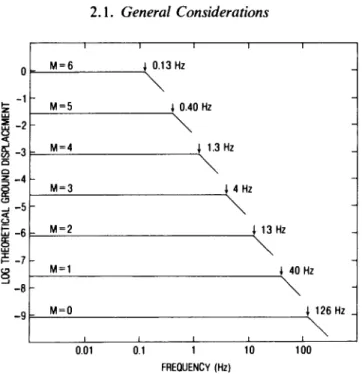
The theoretical spectral amplitudes of ground displacement for earth- quakes from magnitude 0 to 6 are shown in Fig. 4. These theoretical spectra were computed from Eqs. (2.4)-(2.5). The instrumental response of the short-period seismic system used in the USGS Central California Microearthquake Network is shown in Fig. 5. The set of combined dis-
2.1. General Considerations 21
Fig. 4. Theoretical spectral amplitude of ground displacement as a function of frequency for earthquakes ranging in magnitude (M) from 0 to 6. Comer frequencies of these earth- quakes are shown by arrows. Label for the ordinate has been shortened.
I I I I I 1 I
0.01 0.1 I 10 100
FREOUENCY (Hz)
Fig. I. Stylized diagram of displacement amplitude response for the USGS short-period microearthquake system (modified from Eaton, 1977). The numbers along each segment of the curve are in units of decibels per octave.
22 2. Instrumentation Systems
2 -
%
M + 0 - 5
-1-
B
1 -CL:
I
fg 2
- 2 -3 z - 3 - 8 s2 - 4 -
5
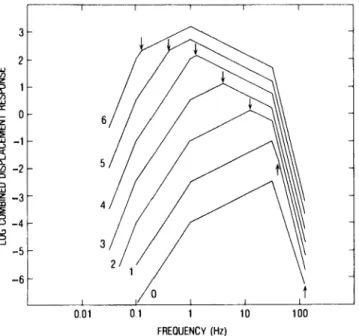
-5placement spectra that would be recorded by the instrumental system is shown in Fig. 6. These are obtained by adding the logarithmic instrumen- tal response curve to each of the logarithmic theoretical ground displace- ment curves. The locations of the theoretical corner frequencies for earth- quakes from magnitude 0 to 6 are shown by arrows in this figure. All the response curves are stylized; each is represented by a small number of linear segments. This is sufficient for the present discussion and is an accepted way to diagram frequency response (Willmore, 1961). The theo- retical ground displacement curves in Fig. 4 do not include the effects of the radiation pattern at the source, absorption and scattering along the transmission path, and conditions at the recording site. These effects are discussed in Thatcher and Hanks (1973).
Some interesting relations can be inferred from the combined displace- ment response curves (Fig. 6). For earthquakes in the magnitude range slightly greater than 1 to about 4, the peak of the combined displacement response curve or, equivalently, the frequency of the maximum amplitude that would be seen on the seismogram, varies with the magnitude of the earthquake. For the assumed source model this frequency corresponds to the corner frequency f o .
-
r
I I I I I3t
-6
1
I I I t
0 01 0 1 1 10 100
FREOUENCY (Hz)
Fig. 6. Theoretical combined displacement response as a function of frequency for earthquakes ranging in magnitude from 0 to 6. Corner frequencies of these earthquakes are shown by arrows, and magnitude of each earthquake is indicated by an integer to the left of each curve.
2.2. Central Califovnia Microearthquake Network 23 Outside of this magnitude range the frequency of the maximum ampli- tude that would be seen on the seismogram does not change. For earth- quakes greater than magnitude 4, the frequency of the maximum ampli- tude will always be 1 Hz. This is caused by (1) the rapid roll-off of the seismometer displacement response below its natural frequency of 1 Hz, and (2) the corner frequency being less than 1 Hz. For earthquakes less than magnitude 1 (assuming that they can be recorded at the 100-km distance assumed here), the frequency of the maximum amplitude will always be 30 Hz. This is caused by ( 1) the rapid roll-off of the response of the seismic amplifier and discriminators above 30 Hz, and (2) the corner frequency being greater than 30 Hz.
2.2. The USGS Central California Microearthquake Network
In 1966 the U.S. Geological Survey began to install a microearthquake network along the San Andreas fault system in central California. The main objective was to develop techniques for mapping microearthquakes in order to study the mechanics of earthquake generation (Eaton et a/., 1970a). The network was designed to telemeter seismic signals from field stations to a recording and processing center in Menlo Park, California.
By early 1980 the network had grown to 250 stations.
Although the basic idea of telemetry transmission and recording has not changed, the instrumentation has been modified since 1966. Major effort has gone into ( 1 ) making the field package low power, compact, long- lived, and weather resistant; (2) increasing signal-to-noise ratio through- out the system; (3) understanding the frequency response of the entire system and its primary components; and (4) improving timing resolution and precision. In cooperative programs with other institutions, equipment similar to that in the USGS Central California Microearthquake Network has been used widely in the United States and some other countries as well. For these reasons we believe that a review of the instrumentation of this network would be instructive.
2.2.1. System Overview
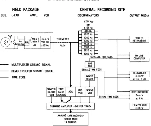
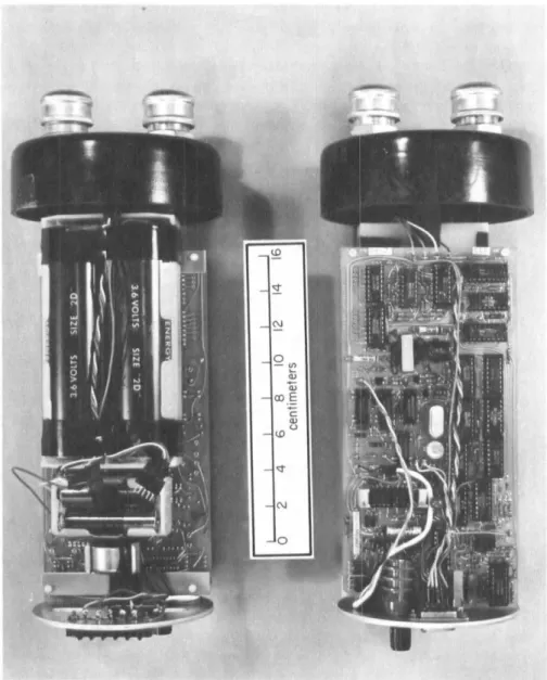
Figure 7 illustrates the major elements of the instrumentation system as currently used. The field package includes a seismometer, amplifier, voltage-controlled oscillator (VCO), frequency stabilizer, automatic daily calibration system, power supply, and telemetry interface. Output from one field package normally is connected to a nearby telephone line drop and transmitted continuously to Menlo Park. A standard voice-grade tele-
24 2. Instrumentation
S
ys terns FIELD PACKAGESEIS. L.PA0 AMPL. VCO
CENTRAL RECORDING SITE
DISCRIMINATORS OUTPUT MEDIA
i2.0 vpp i125H1: per
1700 Hz RETRANSMIT
2040 HI 2380 HI 2720 Hz 3060 tiz
~ f125Hz PATH
ON.LINE COMWTER PARALLEL TIME C O M
-
MULTIPLEXED SEISMIC SIGNAL - DEMULTIPLEXEO SEISMIC SIGNAL~ TIME CODE
HELICOROER 4 cm/V
IGNALS
I
SUMMING AMPLIFIER . ONE PER TRACKI
DIRECT MODE 14 TRACKS
Fig. 7. Major elements of seismic instrumentation of the USGS Central California Mi.
croearthquake Network.
phone circuit with no special conditioning is used. If the field package output cannot be connected to a drop, it is transmitted via line-of-sight vhf radio to a convenient drop and transmitted from there using the telephone system.
As many as eight seismic signals are carried along one voice-grade circuit. This is accomplished by frequency division multiplexing (FDM), as follows. Voice-grade lines transmit audio signals in the frequency range of 30&3300 Hz. In our system of FDM the usable bandwidth is divided into eight FM subcarriers, each with a uniquely specified center fre- quency. A voltage-controlled oscillator in the field package converts the analog signal from the seismometer into a frequency-modulated signal for transmission. Figure 8 shows the eight subcarrier center frequencies used.
The frequencies denoted as TI, T2, and C are not transmitted, and are discussed later. The maximum deviation allowed from each center fre- quency is 5 125 Hz, which corresponds to 53.375 V peak output from the amplifier. A spectrum analyzer monitoring a well-adjusted telemetry line
2.2. Central California Microearthquake Network 25
1 2 3 4 5 6 7 8 11 T2 c Channel
I I 1 I I 1 1 I I I 1
680 1020 1360 1700 2040 2380 2720 3060 3500 3950 4687.5 Ctr Freq (HI) f125 f125 f125 i125 +125 +125 f125 f125 +50 f50 fO Modulalon(HI) f125 f125 f125 ?125 f125 i125 f125 f125 f125 +125 f200 Derodulatwxl(Hz)
I I 1 1 I I I I I I
500 1000 2000 3000 4000 5000
FAEOUENCY (HI)
Fig. 8. Format of frequency division multiplexing (FDM) used for telemetry transmis- sion and recording by the USGS Central California Microearthquake Network (modified from Eaton, 1976).
would show eight spectral peaks, spaced at intervals of 340 Hz and of approximately the same height. The reason for using FDM is to reduce the cost of data transmission.
When the telemetered FDM signal reaches the central recording site, it is divided and sent to two places (Fig. 7). First, it is sent through an automatic gain control (AGC) system, time code and other signals are added to it, and the combined signal is recorded in direct mode on an analog magnetic tape recorder. Second, it is sent through a bank of eight frequency discriminators (matching the eight FDM subcaniers), and the original analog signals are restored. The analog signals may be recorded on paper or photographic film. They may also be sent to an on-line com- puter system or retransmitted to other recording centers.
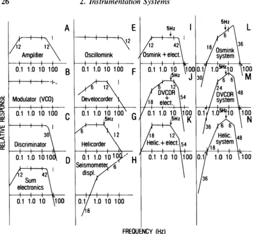
Eaton (1977) summarized the amplitude-frequency response of each of the major components of the USGS telemetry system (Fig. 9). Before proceeding with a summary of the instrumentation, it is instructive to consider how each system component contributes to the response of the entire system. The response curves in Fig. 9 are determined from design and manufacturers’ specifications and from simple tests with a function generator. Each response curve is stylized, with emphasis given to the frequency at which various slopes change and to the rate of attenuation.
Figure 9A-C shows the essential features of the amplitude-frequency response for the major electronic units-the amplifier and VCO in the field package, and the discriminator at the central recording site. The com- bined response of these three units is shown in Fig. 9D and is referred to as the electronics response. The low-frequency roll-off starting at 0. I Hz for the electronics response is due solely to the amplifier in the field package, whereas the high-frequency roll-off starting at 30 Hz has con- tributions from both the amplifier in the field and the discriminator at the central site. Figure 9E-G shows the response of the recording devices- the Oscillomink (a multichannel ink-jet oscillograph), the Develocorder,
26 2. lrrstrumentcition Systems
Modulator (VCO)
-
0.1 1.0 10 100c
1 1 1
0.1 1.0 lolod,
D
E
Oscillomink
FREOl
‘ P6
NCY (Hz)
Fig. 9. Stylized amplitude response of individual components and combinations of com- ponents used in the USGS Central California Microearthquake Network (modified from Eaton, 1977). Amplitude attenuation is shown as an integer in dB/octave.
and the Helicorder. The Oscillomink is used for making high-speed playbacks of earthquakes originally recorded on magnetic tape. It has a flat frequency response from dc to well over 100 Hz. The Develocorder is the primary on-line film recording device. In orde