The scholarship of this book is unparalleled in its area. This text is for inter-connection networks what Hennessy and Patterson’s text is for computer architec-ture — an authoritative, one-stop source that clearly and methodically explains the more significant concepts. Treatment of the material both in breadth and in depth is very well done . . . a must read and a slam dunk! — Timothy Mark Pinkston, Univer-sity of Southern California
[This book is] the most comprehensive and coherent work on modern intercon-nection networks. As leaders in the field, Dally and Towles capitalize on their vast experience as researchers and engineers to present both the theory behind such net-works and the practice of building them. This book is a necessity for anyone studying, analyzing, or designing interconnection networks. — Stephen W. Keckler, The Uni-versity of Texas at Austin
This book will serve as excellent teaching material, an invaluable research refer-ence, and a very handy supplement for system designers. In addition to documenting and clearly presenting the key research findings, the book’s incisive practical treat-ment is unique. By presenting how actual design constraints impact each facet of interconnection network design, the book deftly ties theoretical findings of the past decades to real systems design. This perspective is critically needed in engineering education. — Li-Shiuan Peh, Princeton University
Principles and Practices of Interconnection Networks is a triple threat: compre-hensive, well written and authoritative. The need for this book has grown with the increasing impact of interconnects on computer system performance and cost. It will be a great tool for students and teachers alike, and will clearly help practicing engineers build better networks. — Steve Scott, Cray, Inc.
Dally and Towles use their combined three decades of experience to create a book that elucidates the theory and practice of computer interconnection networks. On one hand, they derive fundamentals and enumerate design alternatives. On the other, they present numerous case studies and are not afraid to give their experi-enced opinions on current choices and future trends. This book is a "must buy" for those interested in or designing interconnection networks. — Mark Hill, University of Wisconsin, Madison
Interconnection Networks
William James Dally
Publishing Services Manager: Simon Crump
Project Manager: Marcy Barnes-Henrie
Editorial Coordinator: Alyson Day
Editorial Assistant: Summer Block
Cover Design: Hannus Design Associates
Cover Image: Frank Stella, Takht-i-Sulayan-I (1967) Text Design: Rebecca Evans & Associates
Composition: Integra Software Services Pvt., Ltd.
Copyeditor: Catherine Albano
Proofreader: Deborah Prato
Indexer: Sharon Hilgenberg
Interior printer The Maple-Vail Book Manufacturing Group
Cover printer Phoenix Color Corp.
Morgan Kaufmann Publishers is an imprint of Elsevier 500 Sansome Street, Suite 400, San Francisco, CA 94111 This book is printed on acid-free paper.
c
2004 by Elsevier, Inc. All rights reserved.
Figure 3.10 c2003 Silicon Graphics, Inc. Used by permission. All rights reserved.
Figure 3.13 courtesy of the Association for Computing Machinery (ACM), from James Laudon and Daniel Lenoski, “The SGI Origin: a ccNUMA highly scalable server,” Proceedings of the International Symposium on Computer Architecture (ISCA), pp. 241-251, 1997. (ISBN: 0897919017) Figure 10. Figure 10.7 from Thinking Machines Corp.
Figure 11.5 courtesy of Ray Mains, Ray Mains Photography, http://www.mauigateway.com/∼raymains/.
Designations used by companies to distinguish their products are often claimed as trademarks or registered trademarks. In all instances in which Morgan Kaufmann Publishers is aware of a claim, the product names appear in initial capital or all capital letters. Readers, however, should contact the appropriate companies for more complete information regarding trademarks and registration. No part of this publication may be reproduced, stored in a retrieval system, or transmitted in any form or by any means—electronic, mechanical, photocopying, or otherwise—without written permission of the publishers.
Permissions may be sought directly from Elsevier’s Science & Technology Rights Department in Oxford, UK: phone: (+44) 1865 843830, fax: (+44) 1865 853333, e-mail:
[email protected]. You may also complete your request on-line via the Elsevier homepage (http://elsevier.com) by selecting "Customer Support" and then "Obtaining Permissions."
Library of Congress Cataloging-in-Publication Data
Dally, William J.
Principles and practices of interconnection networks / William Dally, Brian Towles.
p. cm.
Includes bibliographical references and index. ISBN 0-12-200751-4 (alk. paper)
1. Computer networks-Design and construction. 2. Multiprocessors. I. Towles, Brian. II. Title. TK5105.5.D3272003
004.6’5–dc22
ISBN: 0-12-200751-4 2003058915
For information on all Morgan Kaufmann publications, visit our Web Site atwww.mkp.com
Printed in the United States of America
Acknowledgments
xvii
Preface
xix
About the Authors
xxv
Chapter 1
Introduction to Interconnection Networks
1
1.1 Three Questions About Interconnection Networks 21.2 Uses of Interconnection Networks 4
1.2.1 Processor-Memory Interconnect 5 1.2.2 I/O Interconnect 8
1.2.3 Packet Switching Fabric 11
1.3 Network Basics 13
1.3.1 Topology 13 1.3.2 Routing 16 1.3.3 Flow Control 17 1.3.4 Router Architecture 19
1.3.5 Performance of Interconnection Networks 19
1.4 History 21
1.5 Organization of this Book 23
Chapter 2
A Simple Interconnection Network
25
2.1 Network Specifications and Constraints 25
2.2 Topology 27
2.3 Routing 31
2.4 Flow Control 32
2.5 Router Design 33
2.6 Performance Analysis 36
2.7 Exercises 42
Chapter 3
Topology Basics
45
3.1 Nomenclature 46
3.1.1 Channels and Nodes 46
3.1.2 Direct and Indirect Networks 47 3.1.3 Cuts and Bisections 48
3.1.4 Paths 48 3.1.5 Symmetry 49
3.2 Traffic Patterns 50
3.3 Performance 51
3.3.1 Throughput and Maximum Channel Load 51 3.3.2 Latency 55
3.3.3 Path Diversity 57
3.4 Packaging Cost 60
3.5 Case Study: The SGI Origin 2000 64
3.6 Bibliographic Notes 69
3.7 Exercises 69
Chapter 4
Butterfly Networks
75
4.1 The Structure of Butterfly Networks 75
4.2 Isomorphic Butterflies 77
4.3 Performance and Packaging Cost 78
4.4 Path Diversity and Extra Stages 81
4.5 Case Study: The BBN Butterfly 84
4.6 Bibliographic Notes 86
4.7 Exercises 86
Chapter 5
Torus Networks
89
5.1 The Structure of Torus Networks 90
5.2 Performance 92
5.2.1 Throughput 92 5.2.2 Latency 95 5.2.3 Path Diversity 96
5.3 Building Mesh and Torus Networks 98
5.4 Express Cubes 100
5.5 Case Study: The MIT J-Machine 102
5.6 Bibliographic Notes 106
Chapter 6
Non-Blocking Networks
111
6.1 Non-Blocking vs. Non-Interfering Networks 112
6.2 Crossbar Networks 112
6.3 Clos Networks 116
6.3.1 Structure and Properties of Clos Networks 116 6.3.2 Unicast Routing on Strictly Non-Blocking
Clos Networks 118
6.3.3 Unicast Routing on Rearrangeable Clos Networks 122 6.3.4 Routing Clos Networks Using Matrix
Decomposition 126
6.3.5 Multicast Routing on Clos Networks 128
6.3.6 Clos Networks with More Than Three Stages 133
6.4 Beneˇs Networks 134
6.5 Sorting Networks 135
6.6 Case Study: The Velio VC2002 (Zeus) Grooming Switch 137
6.7 Bibliographic Notes 142
6.8 Exercises 142
Chapter 7
Slicing and Dicing
145
7.1 Concentrators and Distributors 146
7.1.1 Concentrators 146 7.1.2 Distributors 148
7.2 Slicing and Dicing 149
7.2.1 Bit Slicing 149 7.2.2 Dimension Slicing 151 7.2.3 Channel Slicing 152
7.3 Slicing Multistage Networks 153
7.4 Case Study: Bit Slicing in the Tiny Tera 155
7.5 Bibliographic Notes 157
7.6 Exercises 157
Chapter 8
Routing Basics
159
8.1 A Routing Example 160
8.2 Taxonomy of Routing Algorithms 162
8.3 The Routing Relation 163
8.4 Deterministic Routing 164
8.5 Case Study: Dimension-Order Routing in the Cray T3D 168
8.6 Bibliographic Notes 170
8.7 Exercises 171
Chapter 9
Oblivious Routing
173
9.1 Valiant’s Randomized Routing Algorithm 174
9.1.1 Valiant’s Algorithm on Torus Topologies 174 9.1.2 Valiant’s Algorithm on Indirect Networks 175
9.2 Minimal Oblivious Routing 176
9.2.1 Minimal Oblivious Routing on a Folded Clos (Fat Tree) 176
9.2.2 Minimal Oblivious Routing on a Torus 178
9.3 Load-Balanced Oblivious Routing 180
9.4 Analysis of Oblivious Routing 180
9.5 Case Study: Oblivious Routing in the
Avici Terabit Switch Router(TSR) 183
9.6 Bibliographic Notes 186
9.7 Exercises 187
Chapter 10
Adaptive Routing
189
10.1 Adaptive Routing Basics 189
10.2 Minimal Adaptive Routing 192
10.3 Fully Adaptive Routing 193
10.4 Load-Balanced Adaptive Routing 195
10.5 Search-Based Routing 196
10.6 Case Study: Adaptive Routing in the
Thinking Machines CM-5 196
10.7 Bibliographic Notes 201
10.8 Exercises 201
Chapter 11
Routing Mechanics
203
11.1 Table-Based Routing 203
11.1.1 Source Routing 204 11.1.2 Node-Table Routing 208
11.2 Algorithmic Routing 211
11.3 Case Study: Oblivious Source Routing in the
11.4 Bibliographic Notes 217
11.5 Exercises 217
Chapter 12
Flow Control Basics
221
12.1 Resources and Allocation Units 222
12.2 Bufferless Flow Control 225
12.3 Circuit Switching 228
12.4 Bibliographic Notes 230
12.5 Exercises 230
Chapter 13
Buffered Flow Control
233
13.1 Packet-Buffer Flow Control 234
13.2 Flit-Buffer Flow Control 237
13.2.1 Wormhole Flow Control 237 13.2.2 Virtual-Channel Flow Control 239
13.3 Buffer Management and Backpressure 245
13.3.1 Credit-Based Flow Control 245 13.3.2 On/Off Flow Control 247 13.3.3 Ack/Nack Flow Control 249
13.4 Flit-Reservation Flow Control 251
13.4.1 A Flit-Reservation Router 252 13.4.2 Output Scheduling 253 13.4.3 Input Scheduling 255
13.5 Bibliographic Notes 256
13.6 Exercises 256
Chapter 14
Deadlock and Livelock
257
14.1 Deadlock 258
14.1.1 Agents and Resources 258 14.1.2 Wait-For and Holds Relations 259 14.1.3 Resource Dependences 260 14.1.4 Some Examples 260
14.1.5 High-Level (Protocol) Deadlock 262
14.2 Deadlock Avoidance 263
14.2.1 Resource Classes 263
14.3 Adaptive Routing 272
14.3.1 Routing Subfunctions and Extended Dependences 272
14.3.2 Duato’s Protocol for Deadlock-Free Adaptive Algorithms 276
14.4 Deadlock Recovery 277
14.4.1 Regressive Recovery 278 14.4.2 Progressive Recovery 278
14.5 Livelock 279
14.6 Case Study: Deadlock Avoidance in the Cray T3E 279
14.7 Bibliographic Notes 281
14.8 Exercises 282
Chapter 15
Quality of Service
285
15.1 Service Classes and Service Contracts 285
15.2 Burstiness and Network Delays 287
15.2.1 (σ, ρ)Regulated Flows 287 15.2.2 Calculating Delays 288
15.3 Implementation of Guaranteed Services 290
15.3.1 Aggregate Resource Allocation 291 15.3.2 Resource Reservation 292
15.4 Implementation of Best-Effort Services 294
15.4.1 Latency Fairness 294 15.4.2 Throughput Fairness 296
15.5 Separation of Resources 297
15.5.1 Tree Saturation 297
15.5.2 Non-interfering Networks 299
15.6 Case Study: ATM Service Classes 299
15.7 Case Study: Virtual Networks in the Avici TSR 300
15.8 Bibliographic Notes 302
15.9 Exercises 303
Chapter 16
Router Architecture
305
16.1 Basic Router Architecture 305
16.1.1 Block Diagram 305 16.1.2 The Router Pipeline 308
16.2 Stalls 310
16.3 Closing the Loop with Credits 312
16.4 Reallocating a Channel 313
16.6 Flit and Credit Encoding 319
16.7 Case Study: The Alpha 21364 Router 321
16.8 Bibliographic Notes 324
16.9 Exercises 324
Chapter 17
Router Datapath Components
325
17.1 Input Buffer Organization 325
17.1.1 Buffer Partitioning 326
17.1.2 Input Buffer Data Structures 328 17.1.3 Input Buffer Allocation 333
17.2 Switches 334
17.2.1 Bus Switches 335 17.2.2 Crossbar Switches 338 17.2.3 Network Switches 342
17.3 Output Organization 343
17.4 Case Study: The Datapath of the IBM Colony
Router 344
17.5 Bibliographic Notes 347
17.6 Exercises 348
Chapter 18
Arbitration
349
18.1 Arbitration Timing 349
18.2 Fairness 351
18.3 Fixed Priority Arbiter 352
18.4 Variable Priority Iterative Arbiters 354
18.4.1 Oblivious Arbiters 354 18.4.2 Round-Robin Arbiter 355 18.4.3 Grant-Hold Circuit 355
18.4.4 Weighted Round-Robin Arbiter 357
18.5 Matrix Arbiter 358
18.6 Queuing Arbiter 360
18.7 Exercises 362
Chapter 19
Allocation
363
19.1 Representations 363
19.2 Exact Algorithms 366
19.3 Separable Allocators 367
19.3.1 Parallel Iterative Matching 371 19.3.2 iSLIP 371
19.4 Wavefront Allocator 373
19.5 Incremental vs. Batch Allocation 376
19.6 Multistage Allocation 378
19.7 Performance of Allocators 380
19.8 Case Study: The Tiny Tera Allocator 383
19.9 Bibliographic Notes 385
19.10 Exercises 386
Chapter 20
Network Interfaces
389
20.1 Processor-Network Interface 390
20.1.1 Two-Register Interface 391 20.1.2 Register-Mapped Interface 392 20.1.3 Descriptor-Based Interface 393 20.1.4 Message Reception 393
20.2 Shared-Memory Interface 394
20.2.1 Processor-Network Interface 395 20.2.2 Cache Coherence 397
20.2.3 Memory-Network Interface 398
20.3 Line-Fabric Interface 400
20.4 Case Study: The MIT M-Machine Network Interface 403
20.5 Bibliographic Notes 407
20.6 Exercises 408
Chapter 21
Error Control
411
21.1 Know Thy Enemy: Failure Modes and Fault Models 411 21.2 The Error Control Process: Detection, Containment,
and Recovery 414
21.3 Link Level Error Control 415
21.3.1 Link Monitoring 415
21.3.2 Link-Level Retransmission 416 21.3.3 Channel Reconfiguration, Degradation,
and Shutdown 419
21.4 Router Error Control 421
21.5 Network-Level Error Control 422
21.6 End-to-end Error Control 423
21.7 Bibliographic Notes 423
Chapter 22
Buses
427
22.1 Bus Basics 428
22.2 Bus Arbitration 432
22.3 High Performance Bus Protocol 436
22.3.1 Bus Pipelining 436
22.3.2 Split-Transaction Buses 438 22.3.3 Burst Messages 439
22.4 From Buses to Networks 441
22.5 Case Study: The PCI Bus 443
22.6 Bibliographic Notes 446
22.7 Exercises 446
Chapter 23
Performance Analysis
449
23.1 Measures of Interconnection Network Performance 449
23.1.1 Throughput 452 23.1.2 Latency 455 23.1.3 Fault Tolerance 456
23.1.4 Common Measurement Pitfalls 456
23.2 Analysis 460
23.2.1 Queuing Theory 461 23.2.2 Probabilistic Analysis 465
23.3 Validation 467
23.4 Case Study: Efficiency and Loss in the
BBN Monarch Network 468
23.5 Bibliographic Notes 470
23.6 Exercises 471
Chapter 24
Simulation
473
24.1 Levels of Detail 473
24.2 Network Workloads 475
24.2.1 Application-Driven Workloads 475 24.2.2 Synthetic Workloads 476
24.3 Simulation Measurements 478
24.3.1 Simulator Warm-Up 479 24.3.2 Steady-State Sampling 481 24.3.3 Confidence Intervals 482
24.4 Simulator Design 484
24.4.3 Random Number Generation 490 24.4.4 Troubleshooting 491
24.5 Bibliographic Notes 491
24.6 Exercises 492
Chapter 25
Simulation Examples
495
25.1 Routing 495
25.1.1 Latency 496
25.1.2 Throughput Distributions 499
25.2 Flow Control Performance 500
25.2.1 Virtual Channels 500 25.2.2 Network Size 502 25.2.3 Injection Processes 503 25.2.4 Prioritization 505 25.2.5 Stability 507
25.3 Fault Tolerance 508
Appendix A
Nomenclature
511
Appendix B
Glossary
515
Appendix C
Network Simulator
521
Bibliography
523
We are deeply indebted to a large number of people who have contributed to the creation of this book. Timothy Pinkston at USC and Li-Shiuan Peh at Princeton were the first brave souls (other than the authors) to teach courses using drafts of this text. Their comments have greatly improved the quality of the finished book. Mitchell Gusat, Mark Hill, Li-Shiuan Peh, Timothy Pinkston, and Craig Stunkel carefully reviewed drafts of this manuscript and provided invaluable comments that led to numerous improvements.
Many people (mostly designers of the original networks) contributed tion to the case studies and verfied their accuracy. Randy Rettberg provided informa-tion on the BBN Butterfly and Monarch. Charles Leiserson and Bradley Kuszmaul filled in the details of the Thinking Machines CM-5 network. Craig Stunkel and Bu-lent Abali provided information on the IBM SP1 and SP2. Information on the Alpha 21364 was provided by Shubu Mukherjee. Steve Scott provided information on the Cray T3E. Greg Thorson provided the pictures of the T3E.
Much of the development of this material has been influenced by the students and staff that have worked with us on interconnection network research projects at Stanford and MIT, including Andrew Chien, Scott Wills, Peter Nuth, Larry Dennison, Mike Noakes, Andrew Chang, Hiromichi Aoki, Rich Lethin, Whay Lee, Li-Shiuan Peh, Jin Namkoong, Arjun Singh, and Amit Gupta.
This material has been developed over the years teaching courses on intercon-nection networks: 6.845 at MIT and EE482B at Stanford. The students in these classes helped us hone our understanding and presentation of the material. Past TAs for EE482B Li-Shiuan Peh and Kelly Shaw deserve particular thanks.
We have learned much from discussions with colleagues over the years, includ-ing Jose Duato (Valencia), Timothy Pinkston (USC), Sudha Yalamanchili (Georgia Tech),Anant Agarwal (MIT),Tom Knight (MIT), Gill Pratt (MIT), Steve Ward (MIT), Chuck Seitz (Myricom), and Shubu Mukherjee (Intel). Our practical understanding of interconnection networks has benefited from industrial collaborations with Justin Rattner (Intel), Dave Dunning (Intel), Steve Oberlin (Cray), Greg Thorson (Cray), Steve Scott (Cray), Burton Smith (Cray), Phil Carvey (BBN and Avici), Larry Den-nison (Avici), Allen King (Avici), Derek Chiou (Avici), Gopalkrishna Ramamurthy (Velio), and Ephrem Wu (Velio).
Denise Penrose, Summer Block, and Alyson Day have helped us throughout the project.
We also thank both Catherine Albano and Deborah Prato for careful editing, and our production manager, Marcy Barnes-Henrie, who shepherded the book through the sometimes difficult passage from manuscript through finished product.
Digital electronic systems of all types are rapidly becoming commmunication lim-ited. Movement of data, not arithmetic or control logic, is the factor limiting cost, performance, size, and power in these systems. At the same time, buses, long the mainstay of system interconnect, are unable to keep up with increasing performance requirements.
Interconnection networksoffer an attractive solution to this communication cri-sis and are becoming pervasive in digital systems. A well-designed interconnection network makes efficient use of scarce communication resources — providing high-bandwidth, low-latency communication between clients with a minimum of cost and energy.
Historically used only in high-end supercomputers and telecom switches, in-terconnection networks are now found in digital systems of all sizes and all types. They are used in systems ranging from large supercomputers to small embedded systems-on-a-chip (SoC) and in applications including inter-processor communi-cation, processor-memory interconnect, input/output and storage switches, router fabrics, and to replace dedicated wiring.
Indeed, as system complexity and integration continues to increase, many design-ers are finding it more efficient to route packets, not wires. Using an interconnection network rather than dedicated wiring allows scarce bandwidth to be shared so it can be used efficiently with a high duty factor. In contrast, dedicated wiring is idle much of the time. Using a network also enforces regular, structured use of communication resources, making systems easier to design, debug, and optimize.
The basic principles of interconnection networks are relatively simple and it is easy to design an interconnection network that efficiently meets all of the require-ments of a given application. Unfortunately, if the basic principles are not under-stood it is also easy to design an interconnection network that works poorly if at all. Experienced engineers have designed networks that have deadlocked, that have per-formance bottlenecks due to a poor topology choice or routing algorithm, and that realize only a tiny fraction of their peak performance because of poor flow control. These mistakes would have been easy to avoid if the designers had understood a few simple principles.
and shared-memory), Internet routers, telecom circuit switches, and I/O intercon-nect. These systems have been designed around a variety of topologies including crossbars, tori, Clos networks, and butterflies. We developed wormhole routing and virtual-channel flow control. In designing these systems and developing these meth-ods we learned many lessons about what works and what doesn’t. In this book, we share with you, the reader, the benefit of this experience in the form of a set of sim-ple princisim-ples for interconnection network design based on topology, routing, flow control, and router architecture.
Organization
The book starts with two introductory chapters and is then divided into five parts that deal with topology, routing, flow control, router architecture, and performance. A graphical outline of the book showing dependences between sections and chap-ters is shown in Figure 1. We start in Chapter 1 by describing what interconnection networks are, how they are used, the performance requirements of their different applications, and how design choices of topology, routing, and flow control are made to satisfy these requirements. To make these concepts concrete and to motivate the remainder of the book, Chapter 2 describes a simple interconnection network in de-tail: from the topology down to the Verilog for each router. The detail of this example demystifies the abstract topics of routing and flow control, and the performance is-sues with this simple network motivate the more sophisticated methods and design approaches described in the remainder of the book.
The first step in designing an interconnection network is to select a topology that meets the throughput, latency, and cost requirements of the application given a set of packaging constraints. Chapters 3 through 7 explore the topology design space. We start in Chapter 3 by developing topology metrics. A topology’s bisection bandwidth and diameter bound its achievable throughput and latency, respectively, and its path diversity determines both performance under adversarial traffic and fault tolerance. Topology is constrained by the available packaging technology and cost requirements with both module pin limitations and system wire bisection governing achievable channel width. In Chapters 4 through 6, we address the performance metrics and packaging constraints of several common topologies: butterflies, tori, and non-blocking networks. Our discussion of topology ends at Chapter 7 with coverage of concentration and toplogy slicing, methods used to handle bursty traffic and to map topologies to packaging modules.
Topology
& Livelock 15. Quality of Service
routing algorithms in Chapter 9 and adaptive routing algorithms in Chapter 10. The routing portion of the book then concludes with a discussion of routing mechanics in Chapter 11.
A flow-control mechanism sequences packets along the path from source to des-tination by allocating channel bandwidth and buffer capacity along the way. A good flow-control mechanism avoids idling resources or blocking packets on resource con-straints, allowing it to realize a large fraction of the potential throughput and minimiz-ing latency respectively. A bad flow-control mechanism may squander throughput by idling resources, increase latency by unnecessarily blocking packets, and may even result in deadlock or livelock. These topics are explored in Chapters 12 through 15. The policies embedded in a routing algorithm and flow-control method are re-alized in a router. Chapters 16 through 22 describe the microarchitecture of routers and network interfaces. In these chapters, we introduce the building blocks of routers and show how they are composed. We then show how a router can be pipelined to handle a flit or packet each cycle. Special attention is given to problems ofarbitration andallocationin Chapters 18 and 19 because these functions are critical to router performance.
To bring all of these topics together, the book closes with a discussion of net-work performance in Chapters 23 through 25. In Chapter 23 we start by defining the basic performance measures and point out a number of common pitfalls that can result in misleading measurements. We go on to introduce the use of queueing theory and probablistic analysis in predicting the performance of interconnection networks. In Chapter 24 we describe how simulation is used to predict network performance covering workloads, measurement methodology, and simulator design. Finally, Chapter 25 gives a number of example performance results.
Teaching Interconnection Networks
The authors have used the material in this book to teach graduate courses on inter-connection networks for over 10 years at MIT (6.845) and Stanford (EE482b). Over the years the class notes for these courses have evolved and been refined. The result is this book.
A one quarter or one semester course on interconnection networks can follow the outline of this book, as indicated in Figure 1. An individual instructor can add or delete the optional chapters (shown to the right side of the shaded area) to tailor the course to their own needs.
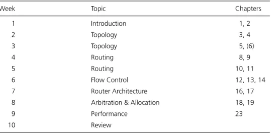
Table 1 One schedule for a ten-week quarter course on interconnection networks. Each chapter covered corresponds roughly to one lecture. In week 3, Chapter 6 through Section 6.3.1 is covered.
Week Topic Chapters
1 Introduction 1, 2
2 Topology 3, 4
3 Topology 5, (6)
4 Routing 8, 9
5 Routing 10, 11
6 Flow Control 12, 13, 14
7 Router Architecture 16, 17
8 Arbitration & Allocation 18, 19
9 Performance 23
10 Review
for students. They see the interplay of the different aspects of interconnection net-work design and get to apply the principles they have learned first hand.
Bill Dally received his B.S. in electrical engineering from Virginia Polytechnic In-stitute, an M.S. in electrical engineering from Stanford University, and a Ph.D. in computer science from Caltech. Bill and his group have developed system architec-ture, network architecarchitec-ture, signaling, routing, and synchronization technology that can be found in most large parallel computers today. While at Bell Telephone Lab-oratories, Bill contributed to the design of the BELLMAC32 microprocessor and designed the MARS hardware accelerator. At Caltech he designed the MOSSIM Simulation Engine and the Torus Routing Chip, which pioneered wormhole routing and virtual-channel flow control. While a Professor of Electrical Engineering and Computer Science at the Massachusetts Institute of Technology, his group built the J-Machine and the M-Machine, experimental parallel computer systems that pio-neered the separation of mechanisms from programming models and demonstrated very low overhead synchronization and communication mechanisms. Bill is currently a professor of electrical engineering and computer science at Stanford University. His group at Stanford has developed the Imagine processor, which introduced the con-cepts of stream processing and partitioned register organizations. Bill has worked with Cray Research and Intel to incorporate many of these innovations in commer-cial parallel computers. He has also worked with Avici Systems to incorporate this technology into Internet routers, and co-founded Velio Communications to com-mercialize high-speed signaling technology. He is a fellow of the IEEE, a fellow of the ACM, and has received numerous honors including the ACM Maurice Wilkes award. He currently leads projects on high-speed signaling, computer architecture, and network architecture. He has published more than 150 papers in these areas and is an author of the textbookDigital Systems Engineering(Cambridge University Press, 1998).
Brian Towles received a B.CmpE in computer engineering from the Georgia Institute of Technology in 1999 and an M.S. in electrical engineering from Stanford University in 2002. He is currently working toward a Ph.D. in electrical engineer-ing at Stanford University. His research interests include interconnection networks, network algorithms, and parallel computer architecture.
Introduction to
Interconnection Networks
Digital systems are pervasive in modern society. Digital computers are used for tasks ranging from simulating physical systems to managing large databases to preparing documents. Digital communication systems relay telephone calls, video signals, and Internet data. Audio and video entertainment is increasingly being delivered and processed in digital form. Finally, almost all products from automobiles to home appliances are digitally controlled.
A digital system is composed of three basic building blocks: logic, memory, and communication. Logic transforms and combines data — for example, by performing arithmetic operations or making decisions. Memory stores data for later retrieval, moving it in time. Communication moves data from one location to another. This book deals with the communication component of digital systems. Specifically, it exploresinterconnection networksthat are used to transport data between the subsys-tems of a digital system.
The performance of most digital systems today is limited by their communication or interconnection, not by their logic or memory. In a high-end system, most of the power is used to drive wires and most of the clock cycle is spent on wire delay, not gate delay. As technology improves, memories and processors become small, fast, and inexpensive. The speed of light, however, remains unchanged. The pin density and wiring density that govern interconnections between system components are scaling at a slower rate than the components themselves. Also, the frequency of communication between components is lagging far beyond the clock rates of modern processors. These factors combine to make interconnection the key factor in the success of future digital systems.
As designers strive to make more efficient use of scarce interconnection bandwidth, interconnection networks are emerging as a nearly universal solution to the system-level communication problems for modern digital systems. Originally
developed for the demanding communication requirements of multicomputers, interconnection networks are beginning to replace buses as the standard system-level interconnection. They are also replacing dedicated wiring in special-purpose systems as designers discover that routing packets is both faster and more economical than routing wires.
1.1
Three Questions About Interconnection Networks
Before going any further, we will answer some basic questions about interconnection networks: What is an interconnection network? Where do you find them? Why are they important?
What is an interconnection network?As illustrated in Figure 1.1, an interconnec-tion network is a programmable system that transports data between terminals. The figure shows six terminals, T1 through T6, connected to a network. When terminal T3 wishes to communicate some data with terminal T5, it sends amessagecontaining the data into the network and the network delivers the message to T5. The network is programmable in the sense that it makes different connections at different points in time. The network in the figure may deliver a message from T3 to T5 in one cycle and then use the same resources to deliver a message from T3 to T1 in the next cycle. The network is a system because it is composed of many components: buffers, channels, switches, and controls that work together to deliver data.
Networks meeting this broad definition occur at many scales. On-chip networks may deliver data between memory arrays, registers, and arithmetic units within a single processor. Board-level and system-level networks tie processors to memories or input ports to output ports. Finally, local-area and wide-area networks connect disparate systems together within an enterprise or across the globe. In this book, we restrict our attention to the smaller scales: from chip-level to system level. Many ex-cellent texts already exist addressing the larger-scale networks. However, the issues at the system level and below, where channels are short and the data rates very
Interconnection network
T1 T2 T3 T4 T5 T6
Figure 1.1 Functional view of an interconnection network.Terminals(labeled T1 through T6) are connected to the network using channels. The arrowheads on each end of the channel indicate it is
high, are fundamentally different than at the large scales and demand different solutions
Where do you find interconnection networks? They are used in almost all digital systems that are large enough to have two components to connect. The most common applications of interconnection networks are in computer systems and communication switches. In computer systems, they connect processors to mem-ories and input/output (I/O) devices to I/O controllers. They connect input ports to output ports in communication switches and network routers. They also connect sensors and actuators to processors in control systems. Anywhere that bits are trans-ported between two components of a system, an interconnection network is likely to be found.
As recently as the late 1980s, most of these applications were served by a very simple interconnection network: the multi-drop bus. If this book had been written then, it would probably be a book on bus design. We devote Chapter 22 to buses, as they are still important in many applications. Today, however, all high-performance interconnections are performed by point-to-point interconnection networks rather than buses, and more systems that have historically been bus-based switch to net-works every year. This trend is due to non-uniform performance scaling. The demand for interconnection performance is increasing with processor performance (at a rate of 50% per year) and network bandwidth. Wires, on the other hand, aren’t getting any faster. The speed of light and the attenuation of a 24-gauge copper wire do not im-prove with better semiconductor technology. As a result, buses have been unable to keep up with the bandwidth demand, and point-to-point interconnection networks, which both operate faster than buses and offer concurrency, are rapidly taking over. Why are interconnection networks important?Because they are a limiting factor in the performance of many systems. The interconnection network between proces-sor and memory largely determines the memory latency and memory bandwidth, two key performance factors, in a computer system.1The performance of the
inter-connection network (sometimes called thefabricin this context) in a communication switch largely determines the capacity (data rate and number of ports) of the switch. Because the demand for interconnection has grown more rapidly than the capability of the underlying wires, interconnection has become a critical bottleneck in most systems.
Interconnection networks are an attractive alternative to dedicated wiring be-cause they allow scarce wiring resources to be shared by several low-duty-factor signals. In Figure 1.1, suppose each terminal needs to communicate one word with each other terminal once every 100 cycles. We could provide a dedicated word-wide channel between each pair of terminals, requiring a total of 30 unidirectional chan-nels. However, each channel would be idle 99% of the time. If, instead, we connect the 6 terminals in a ring, only 6 channels are needed. (T1 connects to T2, T2 to T3, and so on, ending with a connection from T6 to T1.) With the ring network,
the number of channels is reduced by a factor of five and the channel duty factor is increased from 1% to 12.5%.
1.2
Uses of Interconnection Networks
To understand the requirements placed on the design of interconnection networks, it is useful to examine how they are used in digital systems. In this section we examine three common uses of interconnection networks and see how these applications drive network requirements. Specifically, for each application, we will examine how the application determines the following network parameters:
1. The number of terminals
2. Thepeak bandwidthof each terminal 3. Theaverage bandwidthof each terminal 4. The requiredlatency
5. Themessage sizeor a distribution of message sizes 6. Thetraffic pattern(s)expected
7. The requiredquality of service
8. The required reliability and availability of the interconnection network We have already seen that the number of terminals, orports, in a network corresponds to the number of components that must be connected to the network. In addition to knowing the number of terminals, the designer also needs to know how the terminals will interact with the network.
Each terminal will require a certain amount of bandwidth from the network, usually expressed in bits per second (bit/s). Unless stated otherwise, we assume the terminal bandwidths aresymmetric— that is, the input and output bandwidths of the terminal are equal. Thepeak bandwidth is the maximum data rate that a terminal will request from the network over a short period of time, whereas the average bandwidthis the average date rate that a terminal will require. As illustrated in the following section on the design of processor-memory interconnects, knowing both the peak and average bandwidths becomes important when trying to minimize the implementation cost of the interconnection network.
Message size, the length of a message in bits, is another important design consid-eration. If messages are small, overheads in the network can have a larger impact on performance than in the case where overheads can be amortized over the length of a larger message. In many systems, there are several possible message sizes.
How the messages from each terminal are distributed across all the possible destination terminals defines a network’straffic pattern. For example, each terminal might send messages to all other terminals with equal probability. This is therandom traffic pattern. If, instead, terminals tend to send messages only to other nearby terminals, the underlying network can exploit this spatiallocalityto reduce cost. In other networks, however, it is important that the specifications hold for arbitrary traffic patterns.
Some networks will also requirequality of service(QoS). Roughly speaking, QoS involves the fair allocation of resources under some service policy. For example, when multiple messages are contending for the same resource in the network, this contention can be resolved in many ways. Messages could be served in a first-come, first-served order based on how long they have been waiting for the resource in question. Another approach gives priority to the message that has been in the network the longest. The choice of between these and other allocation policies is based on the services required from the network.
Finally, the reliability and availability required from an interconnection network influence design decisions.Reliabilityis a measure of how often the network correctly performs the task of delivering messages. In most situations, messages need to be delivered 100% of time without loss. Realizing a 100% reliable network can be done by adding specialized hardware to detect and correct errors, a higher-level software protocol, or using a mix of these approaches. It may also be possible for a small fraction of messages to be dropped by the network as we will see in the following section on packet switching fabrics. The availabilityof a network is the fraction of time it is available and operating correctly. In an Internet router, an availability of 99.999% is typically specified — less than five minutes of total downtime per year. The challenge of providing this level availability of is that the components used to implement the network will often fail several times a minute. As a result, the network must be designed to detect and quickly recover from these failures while continuing to operate.
1.2.1
Processor-Memory Interconnect
Figure 1.2 illustrates two approaches of using an interconnection network to connect processors to memories. Figure 1.2(a) shows adance-hallarchitecture2in whichP
processors are connected toMmemory banks by an interconnection network. Most modern machines use the integrated-node configuration shown in Figure 1.2(b),
(a)
Interconnection network P
M P
M
P
M
Interconnection network
P M
C
P M
C
P M
C
(b)
Figure 1.2 Use of an interconnection network to connect processor and memory. (a)Dance-hall architec-ture with separate processor (P) and memory (M) ports. (b) Integrated-node architecarchitec-ture with combined processor and memory ports and local access to one memory bank.
Table 1.1 Parameters of processor-memory interconnection networks.
Parameter Value
Processor ports 1–2,048
Memory ports 0–4,096
Peak bandwidth 8 Gbytes/s
Average bandwidth 400 Mbytes/s
Message latency 100 ns
Message size 64 or 576 bits
Traffic patterns arbitrary
Quality of service none
Reliability no message loss
Availability 0.999 to 0.99999
where processors and memories are combined in an integrated node. With this ar-rangement, each processor can access its local memory via a communication switch C without use of the network.
vector processor has 32 processor ports making requests of 4,096 memory banks. This large ratio maximizes memory bandwidth and reduces the probability ofbank conflicts in which two processors simultaneously require access to the same mem-ory bank.
A modern microprocessor executes about 109instructions per second and each instruction can require two 64-bit words from memory (one for the instruction itself and one for data). If one of these references misses in the caches, a block of 8 words is usually fetched from memory. If we really needed to fetch 2 words from memory each cycle, this would demand a bandwidth of 16 Gbytes/s. Fortunately, only about one third of all instructions reference data in memory, and caches work well to reduce the number of references that must actually reference a memory bank. With typical cache-miss ratios, the average bandwidth is more than an order of magnitude lower — about 400 Mbytes/s.3However, to avoid increasing memory
latency due to serialization, most processors still need to be able to fetch at a peak rate of one word per instruction from the memory system. If we overly restricted this peak bandwidth, a sudden burst of memory requests would quickly clog the processor’s network port. The process of squeezing this high-bandwidth burst of requests through a lower bandwidth network port, analogous to a clogged sink slowly draining, is called serialization and increases message latency. To avoid serialization during bursts of requests, we need a peak bandwidth of 8 Gbytes/s.
Processor performance is very sensitive to memory latency, and hence to the latency of the interconnection network over which memory requests and replies are transported. In Table 1.1, we list a latency requirement of 100 ns because this is the basic latency of a typical memory system without the network. If our net-work adds an additional 100 ns of latency, we have doubled the effective memory latency.
When theloadandstoreinstructions miss in the processor’s cache (and are not addressed to the local memory in the integrated-node configuration) they are con-verted into read-request and write-request packets and forwarded over the network to the appropriate memory bank. Each read-request packet contains the memory address to be read, and each write-request packet contains both the memory address and a word or cache line to be written. After the appropriate memory bank receives a request packet, it performs the requested operation and sends a corresponding read-reply or write-reply packet.4
Notice that we have begun to distinguish between messagesandpacketsin our network. A message is the unit of transfer from the network’s clients — in this case, processors and memories — to the network. At the interface to the network, a single message can create one or more packets. This distinction allows for simplification of the underlying network, as large messages can be broken into several smaller packets, or unequal length messages can be split into fixed length packets. Because
3. However, this average demand isverysensitive to the application. Some applications have very poor locality, resulting in high cache-miss ratios and demands of 2 Gbytes/s or more bandwidth from memory. 4. A machine that runs a cache-coherence protocol over the interconnection network requires several
Read request /
write reply header addr
header addr Read reply/
write request data
0
6364 575
0
63
Figure 1.3 The two packet formats required for the processor-memory interconnect.
of the relatively small messages created in this processor-memory interconnect, we assume a one-to-one correspondence between messages and packets.
Read-request and write-reply packets do not contain any data, but do store an address. This address plus some header and packet type information used by the net-work fits comfortably within 64 bits. Read-reply and write-request packets contain the same 64 bits of header and address information plus the contents of a 512-bit cache line, resulting in 576-bit packets. These two packet formats are illustrated in Figure 1.3.
As is typical with processor-memory interconnect, we do not require any specific QoS. This is because the network is inherentlyself-throttling. That is, if the network becomes congested, memory requests will take longer to be fulfilled. Since the pro-cessors can have only a limited number of requests outstanding, they will begin idle, waiting for the replies. Because the processors are not creating new requests while they are idling, the congestion of the network is reduced. This stabilizing behavior is called self-throttling. Most QoS guarantees affect the network only when it is con-gested, but self-throttling tends to avoid congestion, thus making QoS less useful in processor-memory interconnects.
This application requires an inherently reliable network with no packet loss. Memory request and reply packets cannot be dropped. A dropped request packet will cause a memory operation to hangforever. At the least, this will cause a user program to crash due to a timeout. At the worst, it can bring down the whole system. Reliability can be layered on an unreliable network — for example, by having each network interface retain a copy of every packet transmitted until it is acknowledged and retransmitting when a packet is dropped. (See Chapter 21.) However, this ap-proach often leads to unacceptable latency for a processor-memory interconnect. Depending on the application, a processor-memory interconnect needs availability ranging from three nines (99.9%) to five nines (99.999%).
1.2.2
I/O Interconnect
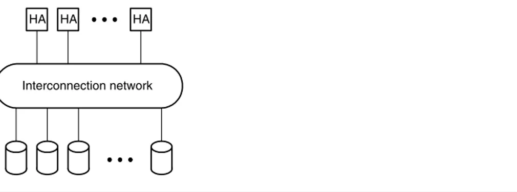
Interconnection network
HA HA HA
Figure 1.4 A typical I/O network connects a number of host adapters to a larger number of I/O devices — in this case, disk drives.
granularity and timing. These differences, particularly an increased latency tolerance, drive the network design in very different directions.
Disk operations are performed by transferringsectorsof 4 Kbytes or more. Due to the rotational latency of the disk plus the time needed to reposition the head, the latency of a sector access may be many milliseconds. A disk read is performed by sending a control packet from a host adapter specifying the disk address (device and sector) to be read and the memory block that is the target of the read. When the disk receives the request, it schedules a head movement to read the requested sector. Once the disk reads the requested sector, it sends a response packet to the appropriate host adapter containing the sector and specifying the target memory block.
The parameters of a high-performance I/O interconnection network are listed in Table 1.2. This network connects up to 64 host adapters and for each host adapter there could be many physical devices, such as hard drives. In this example, there are up to 64 I/O devices per host adapter, for a total of 4,096 devices. More typical systems might connect a few host adapters to a hundred or so devices.
The disk ports have a high ratio of peak-to-average bandwidth. When a disk is transferring consecutive sectors, it can read data at rates of up to 200 Mbytes/s. This number determines the peak bandwidth shown in the table. More typically, the disk must perform a head movement between sectors taking an average of 5 ms (or more), resulting in an average data rate of one 4-Kbyte sector every 5 ms, or less than 1 Mbyte/s. Since the host ports each handle the aggregate traffic from 64 disk ports, they have a lower ratio of peak-to-average bandwidth.
Table 1.2 Parameters of I/O interconnection networks.
Parameter Value
Device ports 1–4,096
Host ports 1–64
Peak bandwidth 200 Mbytes/s
Average bandwidth 1 Mbytes/s (devices)
64 Mbytes/s (hosts)
Message latency 10μs
Message size 32 bytes or 4 Kbytes
Traffic patterns arbitrary
Reliability no message lossa
Availability 0.999 to 0.99999
aA small amount of loss is acceptable, as the error recovery for a failed I/O operation is much more graceful than for a failed memory reference.
“aggregate” port. The average bandwidth of this aggregated port is proportional to the number of devices sharing it. However, because the individual devices infre-quently request their peak bandwidth from the network, it is very unlikely that more than a couple of the many devices are demanding their peak bandwidth from the aggregated port. By concentrating, we have effectively reduced the ratio between the peak and average bandwidth demand, allowing a less expensive implementation without excessive serialization latency.
Like the processor-memory network, the message payload size is bimodal, but with a greater spread between the two modes. The network carries short (32-byte) messages to request read operations, acknowledge write operations, and perform disk control. Read replies and write request messages, on the other hand, require very long (8-Kbyte) messages.
Because the intrinsic latency of disk operations is large (milliseconds) and be-cause the quanta of data transferred as a unit is large (4 Kbyte), the network is not very latency sensitive. Increasing latency to 10μs would cause negligible degradation in performance. This relaxed latency specification makes it much simpler to build an efficient I/O network than to build an otherwise equivalent processor-memory network where latency is at a premium.
Inter-processor communication networks used for fast message passing in cluster-based parallel computers are actually quite similar to I/O networks in terms of their bandwidth and granularity and will not be discussed separately. These networks are often referred to as system-area networks (SANs) and their main difference from I/O networks is more sensitivity to message latency, generally requiring a network with latency less than a few microseconds.
Interconnection network Line
card
Line card
Line card
Figure 1.5 Some network routers use interconnection networks as a switching fabric, passing packets between line cards that transmit and receive packets over network channels.
goes down. It is not unusual for storage systems to have availability of 0.99999 (five nines) — no more than five minutes of downtime per year.
1.2.3
Packet Switching Fabric
Interconnection networks have been replacing buses and crossbars as the switch-ingfabricfor communication network switches and routers. In this application, an interconnection network is acting as an element of a router for a larger-scale net-work (local-area or wide-area). Figure 1.5 shows an example of this application. An array ofline cardsterminates the large-scale network channels (usually optical fibers with 2.5 Gbits/s or 10 Gbits/s of bandwidth).5The line cards process each packet
or cellto determine its destination, verify that it is in compliance with its service agreement, rewrite certain fields of the packet, and update statistics counters. The line card then forwards each packet to the fabric. The fabric is then responsible for forwarding each packet from its source line card to its destination line card. At the destination side, the packet is queued and scheduled for transmission on the output network channel.
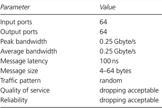
Table 1.3 shows the characteristics of a typical interconnection network used as a switching fabric. The biggest differences between the switch fabric requirements and the processor-memory and I/O network requirements are its high average bandwidth and the need for quality of service.
The large packet size of a switch fabric, along with its latency insensitivity, sim-plifies the network design because latency and message overhead do not have to be highly optimized. The exact packet sizes depend on the protocol used by the
Table 1.3 Parameters of a packet switching fabric.
Parameter Value
Ports 4–512
Peak Bandwidth 10 Gbits/s
Average Bandwidth 7 Gbits/s
Message Latency 10μs
Packet Payload Size 40–64 Kbytes
Traffic Patterns arbitrary
Reliability <10−15loss rate
Quality of Service needed
Availability 0.999 to 0.99999
router. For Internet protocol (IP), packets range from 40 bytes to 64 Kbytes,6with
most packets either 40, 100, or 1,500 bytes in length. Like our other two examples, packets are divided between short control messages and large data transfers.
A network switch fabric isnotself-throttling like the processor-memory or I/O interconnect. Each line card continues to send a steady stream of packets regardless of the congestion in the fabric and, at the same time, the fabric must provide guaranteed bandwidth to certain classes of packets. To meet this service guarantee, the fabric must benon-interfering. That is, an excess in traffic destined for line-carda, perhaps due to a momentary overload, should not interfere with or “steal” bandwidth from traffic destined for a different line cardb, even if messages destined toaand messages destined tobshare resources throughout the fabric. This need for non-interference places unique demands on the underlying implementation of the network switch fabric.
An interesting aspect of a switch fabric that can potentially simplify its design is that in some applications it may be acceptable to drop a very small fraction of pack-ets — say, one in every 1015. This would be allowed in cases where packet dropping is already being performed for other reasons ranging from bit-errors on the input fibers (which typically have an error rate in the 10−12to 10−15range) to overflows in the line card queues. In these cases, a higher-level protocol generally handles dropped packets, so it is acceptable for the router to handle very unlikely circumstances (such as an internal bit error) by dropping the packet in question, as long as the rate of these drops is well below the rate of packet drops due to other reasons. This is in contrast to a processor-memory interconnect, where a single lost packet can lock up the machine.
1.3
Network Basics
To meet the performance specifications of a particular application, such as those described above, the network designer must work within technology constraints to implement thetopology,routing, andflow controlof the network. As we have said in the previous sections, a key to the efficiency of interconnection networks comes from the fact that communication resources are shared. Instead of creating a dedicated channel between each terminal pair, the interconnection network is implemented with a collection of shared router nodes connected by shared channels. The connection pattern of these nodes defines the network’s topology. A message is then delivered between terminals by making several hops across the shared channels and nodes from its source terminal to its destination terminal. A good topology exploits the properties of the network’s packaging technology, such as the number of pins on a chip’s package or the number of cables that can be connected between separate cabinets, to maximize the bandwidth of the network.
Once a topology has been chosen, there can be many possible paths (sequences of nodes and channels) that a message could take through the network to reach its destination. Routing determines which of these possible paths a message actually takes. A good choice of paths minimizes their length, usually measured as the num-ber of nodes or channels visited, while balancing the demand placed on the shared resources of the network. The length of a path obviously influences latency of a message through the network, and the demand orloadon a resource is a measure of how often that resource is being utilized. If one resource becomes over-utilized while another sits idle, known as a load imbalance, the total bandwidth of messages being delivered by the network is reduced.
Flow controldictates which messages get access to particular network resources over time. This influence of flow control becomes more critical as the utilization of resource increases and good flow control forwards packets with minimum delay and avoids idling resources under high loads.
1.3.1
Topology
Interconnection networks are composed of a set of shared router nodes and chan-nels, and the topologyof the network refers to the arrangement of these nodes and channels. The topology of an interconnection network is analogous to a roadmap. The channels (like roads) carry packets (like cars) from one router node (intersection) to another. For example, the network shown in Figure 1.6 consists of 16 nodes, each of which is connected to 8 channels, 1 to each neighbor and 1 from each neighbor. This particular network has atorustopology. In the figure, the nodes are denoted by circles and each pair of channels, one in each direction, is denoted by a line joining two nodes. This topology is also adirect network, where a terminal is associated with each of the 16 nodes of the topology.
00 01 02
10 11 12
20 21 22
03 13 23
30 31 32 33
Figure 1.6 A network topology is the arrangements of nodes, denoted by circles numbered 00 to 33 and channels connecting the nodes. A pair of channels, one in each direction, is denoted by each line in the figure. In this4×4, 2-D torus, or 4-ary 2-cube, topology, each node is connected to 8 channels: 1 channel to and 1 channel from each of its 4 neighbors.
cost. To maximize bandwidth, a topology should saturate thebisection bandwidth, the bandwidth across the midpoint of the system, provided by the underlying packaging technology.
For example, Figure 1.7 shows how the network from Figure 1.6 might be pack-aged. Groups of four nodes are placed on vertical printed circuit boards. Four of the circuit boards are then connected using a backplane circuit board, just as PCI cards might be plugged into the motherboard of a PC. For this system, the bisection bandwidth is the maximum bandwidth that can be transferred across this backplane. Assuming the backplane is wide enough to contain 256 signals, each operating at a data rate of 1 Gbit/s, the total bisection bandwidth is 256 Gbits/s.
Referring back to Figure 1.6, exactly 16 unidirectional channels cross the mid-point of our topology — remember that the lines in the figure represent two channels, one in each direction. To saturate the bisection of 256 signals, each chan-nel crossing the bisection should be 256/16=16 signals wide. However, we must also take into account the fact that each node will be packaged on a single IC chip. For this example, each chip has only enough pins to support 128 signals. Since our topology requires a total of 8 channels per node, each chip’s pin constraint limits the channel width to 128/8 =16 signals. Fortunately, the channel width given by pin limitations exactly matches the number of signals required to saturate the bisection bandwidth.
00 10 20 33 00 10 20 32 00 10 20 31
Backplane
00 10 20 30
PC boards
256 signals
Figure 1.7 A packaging of a 16-node torus topology. Groups of 4 nodes are packaged on single printed circuit boards, four of which are connected to a single backplane board. The backplane channels for the third column are shown along the right edge of the backplane. The number of signals across the width of the backplane (256) defines the bisection bandwidth of this particular package.
0 1 2 3 4 5 6 7
15 14 13 12 11 10 9 8
Figure 1.8 For the constraints of our example, a 16-node ring network has lower latency than the 16-node, 2-D torus of Figure 1.6. This latency is achieved at the expense of lower throughput.
pins limit the channel width to only half of this. Thus, with identical technology constraints, the ring topology provides only half the bandwidth of the torus topology. In terms of bandwidth, the torus is obviously a superior choice, providing the full 32 Gbits/s of bandwidth per node across the midpoint of the system.
However, high bandwidth is not the only measure of a topology’s performance. Suppose we have a different application that requires only 16 Gbits/s of bandwidth under identical technology constraints, but also requires the minimum possible latency. Moreover, suppose this application uses rather long 4,096-bit packets. To achieve a low latency, the topology must balance the desire for a small average dis-tance between nodes against a lowserialization latency.
latency. To see how this tradeoff affects topology choice, we revisit our two 16-node topologies, but now we focus on message latency.
First, to quantify latency due to hop count, a traffic pattern needs to be assumed. For simplicity, we userandom traffic, where each node sends to every other node with equal probability. The average hop count under random traffic is just the average distance between nodes. For our torus topology, the average distance is 2 and for the ring the average distance is 4. In a typical network, the latency per hop might be 20 ns, corresponding to a total hop latency of 40 ns for the torus and 80 ns for the ring.
However, the wide channels of the ring give it a much lower serialization latency. To send a 4,096-bit packet across a 32-signal channel requires 4,096/32 = 128 cycles of the channel. Our signaling rate of 1 GHz corresponds to a period of 1 ns, so the serialization latency of the ring is 128 ns. We have to pay this serialization time only once if our network is designed efficiently, which gives an average delay of 80+128 =208 ns per packet through the ring. Similar calculations for the torus yield a serialization latency of 256 ns and a total delay of 296 ns. Even though the ring has a greater average hop count, the constraints of physical packaging give it a lower latency for these long packets.
As we have seen here, no one topology is optimal for all applications. Different topologies are appropriate for different constraints and requirements. Topology is discussed in more detail in Chapters 3 through 7.
1.3.2
Routing
The routing method employed by a network determines the path taken by a packet from a source terminal node to a destination terminal node. A route or path is an ordered set of channels P = {c1, c2, . . . , ck}, where the output node of channelci equals the input node of channelci+1, the source is the input to channel c1, and the destination is the output of channelck. In some networks there is only a single route from each source to each destination, whereas in others, such as the torus network in Figure 1.6, there are many possible paths. When there are many paths, a good routing algorithm balances the load uniformly across channels regardless of the offered traffic pattern. Continuing our roadmap analogy, while the topology provides the roadmap, the roads and intersections, the routing method steers the car, making the decision on which way to turn at each intersection. Just as in routing cars on a road, it is important to distribute the traffic — to balance the load across different roads rather than having one road become congested while parallel roads are empty.
![Figure 3.11 For up to 16 routers (R) (32 nodes [N]) the Origin 2000 has a binary n-cube topology, n ≤ 4](https://thumb-ap.123doks.com/thumbv2/123dok/4033638.1977058/93.789.143.643.122.504/figure-routers-r-nodes-origin-binary-cube-topology.webp)
