Principles, Methods and Applications
Networks constitute the backbone of complex systems, from the human brain to computer communications, transport infrastructures to online social systems, metabolic reactions to financial markets. Characterising their structure improves our understanding of the physical, biological, economic and social phenomena that shape our world.
Rigorous and thorough, this textbook presents a detailed overview of the new theory and methods of network science. Covering algorithms for graph exploration, node ranking and network generation, among the others, the book allows students to experiment with network models and real-world data sets, providing them with a deep understanding of the basics of network theory and its practical applications. Systems of growing complexity are examined in detail, challenging students to increase their level of skill. An engaging pre-sentation of the important principles of network science makes this the perfect reference for researchers and undergraduate and graduate students in physics, mathematics, engineering, biology, neuroscience and social sciences.
Vito Latorais Professor of Applied Mathematics and Chair of Complex Systems at Queen Mary University of London. Noted for his research in statistical physics and in complex networks, his current interests include time-varying and multiplex networks, and their applications to socio-economic systems and to the human brain.
Vincenzo Nicosiais Lecturer in Networks and Data Analysis at the School of Mathematical Sciences at Queen Mary University of London. His research spans several aspects of net-work structure and dynamics, and his recent interests include multi-layer netnet-works and their applications to big data modelling.
Complex Networks
Principles, Methods and Applications
V I T O L AT O R A
Queen Mary University of LondonV I N C E N Z O N I C O S I A
Queen Mary University of London477 Williamstown Road, Port Melbourne, VIC 3207, Australia 4843/24, 2nd Floor, Ansari Road, Daryaganj, Delhi – 110002, India
79 Anson Road, #06–04/06, Singapore 079906 Cambridge University Press is part of the University of Cambridge. It furthers the University’s mission by disseminating knowledge in the pursuit of education, learning, and research at the highest international levels of excellence.
www.cambridge.org
Information on this title: www.cambridge.org/9781107103184 DOI: 10.1017/9781316216002
© Vito Latora, Vincenzo Nicosia and Giovanni Russo 2017 This publication is in copyright. Subject to statutory exception and to the provisions of relevant collective licensing agreements,
no reproduction of any part may take place without the written permission of Cambridge University Press.
First published 2017
Printed in the United Kingdom by TJ International Ltd. Padstow Cornwall A catalogue record for this publication is available from the British Library.
Library of Congress Cataloging-in-Publication Data
Names: Latora, Vito, author. | Nicosia, Vincenzo, author. | Russo, Giovanni, author. Title: Complex networks : principles, methods and applications / Vito Latora, Queen Mary University of London, Vincenzo Nicosia, Queen Mary University
of London, Giovanni Russo, Università degli Studi di Catania, Italy. Description: Cambridge, United Kingdom ; New York, NY : Cambridge University
Press, 2017. | Includes bibliographical references and index. Identifiers: LCCN 2017026029 | ISBN 9781107103184 (hardback)
Subjects: LCSH: Network analysis (Planning) Classification: LCC T57.85 .L36 2017 | DDC 003/.72–dc23
LC record available at https://lccn.loc.gov/2017026029 ISBN 978-1-107-10318-4 Hardback
Additional resources for this publication at www.cambridge.org/9781107103184. Cambridge University Press has no responsibility for the persistence or accuracy of
URLs for external or third-party internet websites referred to in this publication and does not guarantee that any content on such websites is, or will remain,
Preface pagexi
Introduction xii
The Backbone of a Complex System xii
Complex Networks Are All Around Us xiv
Why Study Complex Networks? xv
Overview of the Book xvii
Acknowledgements xx
1
Graphs and Graph Theory
11.1 What Is a Graph? 1
1.2 Directed, Weighted and Bipartite Graphs 9
1.3 Basic Definitions 13
1.4 Trees 17
1.5 Graph Theory and the Bridges of Königsberg 19
1.6 How to Represent a Graph 23
1.7 What We Have Learned and Further Readings 28
Problems 28
2
Centrality Measures
312.1 The Importance of Being Central 31
2.2 Connected Graphs and Irreducible Matrices 34
2.3 Degree and Eigenvector Centrality 39
2.4 Measures Based on Shortest Paths 47
2.5 Movie Actors 56
2.6 Group Centrality 62
2.7 What We Have Learned and Further Readings 64
Problems 65
3
Random Graphs
693.1 Erd˝os and Rényi (ER) Models 69
3.2 Degree Distribution 76
3.3 Trees, Cycles and Complete Subgraphs 79
3.4 Giant Connected Component 84
3.5 Scientific Collaboration Networks 90
3.6 Characteristic Path Length 94
3.7 What We Have Learned and Further Readings 103
Problems 104
4
Small-World Networks
1074.1 Six Degrees of Separation 107
4.2 The Brain of a Worm 112
4.3 Clustering Coefficient 116
4.4 The Watts–Strogatz (WS) Model 127
4.5 Variations to the Theme 135
4.6 Navigating Small-World Networks 144
4.7 What We Have Learned and Further Readings 148
Problems 148
5
Generalised Random Graphs
1515.1 The World Wide Web 151
5.2 Power-Law Degree Distributions 161
5.3 The Configuration Model 171
5.4 Random Graphs with Arbitrary Degree Distribution 178
5.5 Scale-Free Random Graphs 184
5.6 Probability Generating Functions 188
5.7 What We Have Learned and Further Readings 202
Problems 204
6
Models of Growing Graphs
2066.1 Citation Networks and the Linear Preferential Attachment 206
6.2 The Barabási–Albert (BA) Model 215
6.3 The Importance of Being Preferential and Linear 224
6.4 Variations to the Theme 230
6.5 Can Latecomers Make It? The Fitness Model 241
6.6 Optimisation Models 248
6.7 What We Have Learned and Further Readings 252
Problems 253
7
Degree Correlations
2577.1 The Internet and Other Correlated Networks 257
7.2 Dealing with Correlated Networks 262
7.3 Assortative and Disassortative Networks 268
7.4 Newman’s Correlation Coefficient 275
7.5 Models of Networks with Degree–Degree Correlations 285
7.6 What We Have Learned and Further Readings 290
Problems 291
8
Cycles and Motifs
2948.1 Counting Cycles 294
8.2 Cycles in Scale-Free Networks 303
8.4 Transcription Regulation Networks 316
8.5 Motif Analysis 324
8.6 What We Have Learned and Further Readings 329
Problems 330
9
Community Structure
3329.1 Zachary’s Karate Club 332
9.2 The Spectral Bisection Method 336
9.3 Hierarchical Clustering 342
9.4 The Girvan–Newman Method 349
9.5 Computer Generated Benchmarks 354
9.6 The Modularity 357
9.7 A Local Method 365
9.8 What We Have Learned and Further Readings 369
Problems 371
10 Weighted Networks
37410.1 Tuning the Interactions 374
10.2 Basic Measures 381
10.3 Motifs and Communities 387
10.4 Growing Weighted Networks 393
10.5 Networks of Stocks in a Financial Market 401
10.6 What We Have Learned and Further Readings 407
Problems 408
Appendices
410A.1 Problems, Algorithms and Time Complexity 410
A.2 A Simple Introduction to Computational Complexity 420
A.3 Elementary Data Structures 425
A.4 Basic Operations with Sparse Matrices 440
A.5 Eigenvalue and Eigenvector Computation 444
A.6 Computation of Shortest Paths 452
A.7 Computation of Node Betweenness 462
A.8 Component Analysis 467
A.9 Random Sampling 474
A.10 Erd˝os and Rényi Random Graph Models 485
A.11 The Watts–Strogatz Small-World Model 489
A.12 The Configuration Model 492
A.13 Growing Unweighted Graphs 499
A.14 Random Graphs with Degree–Degree Correlations 506
A.15 Johnson’s Algorithm to Enumerate Cycles 508
A.16 Motifs Analysis 511
A.17 Girvan–Newman Algorithm 515
A.18 Greedy Modularity Optimisation 519
A.20 Kruskal’s Algorithm for Minimum Spanning Tree 528
A.21 Models for Weighted Networks 531
List of Programs 533
References 535
Author Index 550
Social systems, the human brain, the Internet and the World Wide Web are all examples of complex networks, i.e. systems composed of a large number of units interconnected through highly non-trivial patterns of interactions. This book is an introduction to the beau-tiful and multidisciplinary world of complex networks. The readers of the book will be exposed to the fundamental principles, methods and applications of a novel discipline: net-work science. They will learn how to characterise the architecture of a network and model
its growth, and will uncover the principles common to networks from different fields. The book covers a large variety of topics including elements of graph theory, social networks and centrality measures, random graphs, small-world and scale-free networks, models of growing graphs and degree–degree correlations, as well as more advanced topics such as motif analysis, community structure and weighted networks. Each chapter presents its main ideas together with the related mathematical definitions, models and algorithms, and makes extensive use of network data sets to explore these ideas.
The book contains several practical applications that range from determining the role of an individual in a social network or the importance of a player in a football team, to iden-tifying the sub-areas of a nervous systems or understanding correlations between stocks in a financial market.
Thanks to its colloquial style, the extensive use of examples and the accompanying soft-ware tools and network data sets, this book is the ideal university-level textbook for a first module on complex networks. It can also be used as a comprehensive reference for researchers in mathematics, physics, engineering, biology and social sciences, or as a his-torical introduction to the main findings of one of the most active interdisciplinary research fields of the moment.
This book is fundamentally on the structure of complex networks, and we hope it will be followed soon by a second book on the different types of dynamical processes that can take place over a complex network.
Vito Latora Vincenzo Nicosia Giovanni Russo
The Backbone of a Complex System
Imagine you are invited to a party; you observe what happens in the room when the other guests arrive. They start to talk in small groups, usually of two people, then the groups grow in size, they split, merge again, change shape. Some of the people move from one group to another. Some of them know each other already, while others are introduced by mutual friends at the party. Suppose you are also able to track all of the guests and their movements in space; their head and body gestures, the content of their discussions. Each person is different from the others. Some are more lively and act as the centre of the social gathering: they tell good stories, attract the attention of the others and lead the group conversation. Other individuals are more shy: they stay in smaller groups and prefer to listen to the others. It is also interesting to notice how different genders and ages vary between groups. For instance, there may be groups which are mostly male, others which are mostly female, and groups with a similar proportion of both men and women. The topic of each discussion might even depend on the group composition. Then, when food and beverages arrive, the people move towards the main table. They organise into more or less regular queues, so that the shape of the newly formed groups is different. The individuals rearrange again into new groups sitting at the various tables. Old friends, but also those who have just met at the party, will tend to sit at the same tables. Then, discussions will start again during the dinner, on the same topics as before, or on some new topics. After dinner, when the music begins, we again observe a change in the shape and size of the groups, with the formation of couples and the emergence of collective motion as everybody starts to dance.
from nest maintenance to the organisation of food search, without the need for any central control.
Let us consider another example of a complex system, certainly the most representative and beautiful one: the human brain. With around 102billion neurons, each connected by synapses to several thousand other neurons, this is the most complicated organ in our body. Neurons are cells which process and transmit information through electrochemical signals. Although neurons are of different types and shapes, the “integrate-and-fire” mechanism at the core of their dynamics is relatively simple. Each neuron receives synaptic signals, which can be either excitatory or inhibitory, from other neurons. These signals are then integrated and, provided the combined excitation received is larger than a certain threshold, the neuron fires. This firing generates an electric signal, called an action potential, which propagates through synapses to other neurons. Notwithstanding the extreme simplicity of the interactions, the brain self-organises collective behaviours which are difficult to pre-dict from our knowledge of the dynamics of its individual elements. From an avalanche of simple integrate-and-fire interactions, the neurons of the brain are capable of organising a large variety of wonderful emerging behaviours. For instance, sensory neurons coordinate the response of the body to touch, light, sounds and other external stimuli. Motor neurons are in charge of the body’s movement by controlling the contraction or relaxation of the muscles. Neurons of the prefrontal cortex are responsible for reasoning and abstract think-ing, while neurons of the limbic system are involved in processing social and emotional information.
of the system. In practice, what also matters in a complex system, and it matters a lot, is the backboneof the system, or, in other words, the architecture of the network of interac-tions. It is precisely on thesecomplex networks, i.e. on the networks of the various complex systems that populate our world, that we will be focusing in this book.
Complex Networks Are All Around Us
Networks permeate all aspects of our life and constitute the backbone of our modern world. To understand this, think for a moment about what you might do in a typical day. When you get up early in the morning and turn on the light in your bedroom, you are connected to the electrical power grid, a network whose nodes are either power stations or users, while links are copper cables which transport electric current. Then you meet the people of your family. They are part of yoursocial networkwhose nodes are people and links stand for kinship, friendship or acquaintance. When you take a shower and cook your breakfast you are respectively using awater distribution network, whose nodes are water stations, reservoirs, pumping stations and homes, and links are pipes, and agas distribution network. If you go to work by car you are moving in thestreet networkof your city, whose nodes are intersections and links are streets. If you take the underground then you make use of a transportation network, whose nodes are the stations and links are route segments.
When you arrive at your office you turn on your laptop, whose internal circuits form a complicated microscopicnetwork of logic gates, and connect it to theInternet, a worldwide network of computers and routers linked by physical or logical connections. Then you check your emails, which belong to anemail communication network, whose nodes are people and links indicate email exchanges among them. When you meet a colleague, you and your colleague form part of acollaboration network, in which an edge exists between two persons if they have collaborated on the same project or coauthored a paper. Your colleagues tell you that your last paper has got its first hundred citations. Have you ever thought of the fact that your papers belong to acitation network, where the nodes represent papers, and links are citations?
At lunchtime you read the news on the website of your preferred newspaper: in doing this you access theWorld Wide Web, a huge global information network whose nodes are webpages and edges are clickable hyperlinks between pages. You will almost surely then check yourFacebookaccount, a typical example of anonline social network, then maybe have a look at the daily trending topics onTwitter, an information network whose nodes are people and links are the “following” relations.
white waterfall cascading down a cliff, and a stream flowing quietly through a green valley. There is no need to say that “lake”, “waterfall”, “white”, “stream”, “cliff”, “valley” and “green” form anetwork of words associations, in which a link exists between two words if these words are often associated with each other in our minds. Before leaving the office, you book a flight to go to Prague for a conference. Obviously, also theair transportation systemis a network, whose nodes are airports and links are airline routes.
When you drive back home you feel a bit tired and you think of the various networks in our body, from thenetwork of blood vesselswhich transports blood to our organs to the intricate set of relationships among genes and proteins which allow the perfect functioning of the cells of our body. Examples of these genetic networks are the transcription regula-tion networksin which the nodes are genes and links represent transcription regulation of a gene by the transcription factor produced by another gene,protein interaction networks whose nodes are protein and there is a link between two proteins if they bind together to perform complex cellular functions, and metabolic networkswhere nodes are chemicals, and links represent chemical reactions.
During dinner you hear on the news that the total export for your country has decreased by 2.3% this year; the system ofcommercial relationshipsamong countries can be seen as a network, in which links indicate import/export activities. Then you watch a movie on your sofa: you can construct anactor collaboration networkwhere nodes represent movie actors and links are formed if two actors have appeared in the same movie. Exhausted, you go to bed and fall asleep while images of networks of all kinds still twist and dance in your mind, which is, after all, the marvellous combination of the activity of billions of neurons and trillions of synapses in yourbrain network. Yet another network.
Why Study Complex Networks?
In the late 1990s two research papers radically changed our view on complex systems, moving the attention of the scientific community to the study of the architecture of a com-plex system and creating an entire new research field known today asnetwork science. The first paper, authored by Duncan Watts and Steven Strogatz, was published in the journal Naturein 1998 and was aboutsmall-world networks[311]. The second one, onscale-free networks, appeared one year later inScienceand was authored by Albert-László Barabási and Réka Albert [19]. The two papers provided clear indications, from different angles, that:
• the networks of real-world complex systems have non-trivial structures and are very
different from lattices or random graphs, which were instead the standard networks commonly used in all the current models of a complex system.
• some structural properties are universal, i.e. are common to networks as diverse as those
of biological, social and man-made systems.
• the structure of the network plays a major role in the dynamics of a complex system and
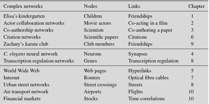
Table 1 A list of the real-world complex networks that will be studied in this book. For each network, we report the chapter of the book where the corresponding data set will be introduced and analysed.
Complex networks Nodes Links Chapter
Elisa’s kindergarten Children Friendships 1
Actor collaboration networks Movie actors Co-acting in a film 2
Co-authorship networks Scientists Co-authoring a paper 3
Citation networks Scientific papers Citations 6
Zachary’s karate club Club members Friendships 9
C. elegansneural network Neurons Synapses 4
Transcription regulation networks Genes Transcription regulation 8
World Wide Web Web pages Hyperlinks 5
Internet Routers Optical fibre cables 7
Urban street networks Street crossings Streets 8
Air transport network Airports Flights 10
Financial markets Stocks Time correlations 10
Both works were motivated by the empirical analysis of real-world systems. Four net-works were introduced and studied in these two papers. Namely, the neural system of a few-millimetres-long worm known as theC. elegans, a social network describing how actors collaborate in movies, and two man-made networks: the US electrical power grid and a sample of the World Wide Web. During the last decade, new technologies and increasing computing power have made new data available and stimulated the exploration of several other complex networks from the real world. A long series of papers has followed, with the analysis of new and ever larger networks, and the introduction of novel measures and models to characterise and reproduce the structure of these real-world systems. Table 1 shows only a small sample of the networks that have appeared in the literature, namely those that will be explicitly studied in this book, together with the chapter where they will be considered. Notice that the table includes different types of networks. Namely, five networks representing three different types of social interactions (namely friendships, collaborations and citations), two biological systems (respectively a neural and a gene net-work) and five man-made networks (from transportation and communication systems to a network of correlations among financial stocks).
The ubiquitousness of networks in nature, technology and society has been the principal motivation behind the systematic quantitative study of their structure, their formation and their evolution. And this is also the main reason why a student of any scientific discipline should be interested in complex networks. In fact, if we want to master the interconnected world we live in, we need to understand the structure of the networks around us. We have to learn the basic principles governing the architecture of networks from different fields, and study how to model their growth.
1995 2000 2005 2010 2015 year
0 2000 4000 6000 8000 10000
# citations
WS BA
1995 2000 2005 2010 2015
year 200
400 600 800
# papers
t
Fig. 1 Left panel: number of citations received over the years by the 1998 Watts and Strogatz (WS) article on small-world networks and by the 1999 Barabási and Albert (BA) article on scale-free networks. Right panel: number of papers on complex networks that appeared each year in the public preprint archive arXiv.org.side by side. Because of its interdisciplinary nature, the generality of the results obtained, and the wide variety of possible applications, network science is considered today a necessary ingredient in the background of any modern scientist.
Finally, it is not difficult to understand that complex networks have become one of the hottest research fields in science. This is confirmed by the attention and the huge number of citations received by Watts and Strogatz, and by Barabási and Albert, in the papers mentioned above. The temporal profiles reported in the left panel of Figure 1 show the exponential increase in the number of citations of these two papers since their publication. The two papers have today about 10,000 citations each and, as already mentioned, have opened a new research field stimulating interest for complex networks in the scientific community and triggering an avalanche of scientific publications on related topics. The right panel of Figure 1 reports the number of papers published each year after 1998 on the well-known public preprint archive arXiv.org with the term “complex networks” in their title or abstract. Notice that this number has gone up by a factor of 10 in the last ten years, with almost a thousand papers on the topic published in the archive in the year 2013. The explosion of interest in complex networks is not limited to the scientific community, but has become a cultural phenomenon with the publications of various popular science books on the subject.
Overview of the Book
The standard tools to study complex networks are a mixture of mathematical and com-putational methods. They require some basic knowledge of graph theory, probability, differential equations, data structures and algorithms, which will be introduced in this book from scratch and in a friendly way. Also, network theory has found many interest-ing applications in several different fields, includinterest-ing social sciences, biology, neuroscience and technology. In the book we have therefore included a large variety of examples to emphasise the power of network science. This book is essentially on the structure of com-plex networks, since we have decided that the detailed treatment of the different types of dynamical processes that can take place over a complex network should be left to another book, which will follow this one.
The book is organised into ten chapters. The first six chapters (Chapters 1–6) form the core of the book. They introduce the main concepts of network science and the basic measures and models used to characterise and reproduce the structure of various com-plex networks. The remaining four chapters (Chapters 7–10) cover more advanced topics that could be skipped by a lecturer who wants to teach a short course based on the book.
In Chapter 1 we introduce some basic definitions from graph theory, setting up the lan-guage we will need for the remainder of the book. The aim of the chapter is to show that complex network theory is deeply grounded in a much older mathematical discipline, namelygraph theory.
In Chapter 2 we focus on the concept of centrality, along with some of the related mea-sures originally introduced in the context ofsocial network analysis, which are today used extensively in the identification of the key components of any complex system, not only of social networks. We will see some of the measures at work, using them to quantify the centrality of movie actors in theactor collaboration network.
Chapter 3 is where we first discuss network models. In this chapter we introduce the classicalrandom graph modelsproposed by Erd˝os and Rényi (ER) in the late 1950s, in which the edges are randomly distributed among the nodes with a uniform probability. This allows us to analytically derive some important properties such as, for instance, the number and order ofgraph componentsin a random graph, and to use ER models as term of comparison to investigatescientific collaboration networks. We will also show that the average distancebetween two nodes in ER random graphs increases only logarithmically with the number of nodes.
In Chapter 4 we see that in real-world systems, such as theneural network of theC. ele-gans or the movie actor collaboration network, the neighbours of a randomly chosen node are directly linked to each other much more frequently than would occur in a purely ran-dom network, giving rise to the presence of many triangles. In order to quantify this, we introduce the so-calledclustering coefficient. We then discuss the Watts and Strogatz (WS) small-world modelto construct networks with both a small average distance between nodes and a high clustering coefficient.
In Chapter 5 the focus is on how the degreekis distributed among the nodes of a network. We start by considering the graph of the World Wide Web and by showing that it is a scale-free network, i.e. it has a power–lawdegree distribution pk∼k−γ with an exponent
γ ∈ [2, 3]. This is a property shared by many other networks, while neither ER random
configuration modelwhich generalises ER random graph models to incorporate arbitrary degree distributions.
In Chapter 6 we show that real networks are not static, but grow over time with the addition of new nodes and links. We illustrate this by studying the basic mechanisms of growth incitation networks. We then consider whether it is possible to produce scale-free degree distributions by modelling the dynamical evolution of the network. For this purpose we introduce theBarabási–Albert model, in which newly arriving nodes select and link existing nodes with a probability linearly proportional to their degree. We also consider some extensions and modifications of this model.
In the last four chapters we cover more advanced topics on the structure of complex networks.
Chapter 7 is about networks withdegree–degree correlations, i.e. networks such that the probability that an edge departing from a node of degreekarrives at a node of degreek′ is a function both ofk′ and ofk. Degree–degree correlations are indeed present in real-world networks, such as theInternet, and can be either positive (assortative) or negative (disassortative). In the first case, networks with small degree preferentially link to other low-degree nodes, while in the second case they link preferentially to high-degree ones. In this chapter we will learn how to take degree–degree correlations into account, and how to model correlated networks.
In Chapter 8 we deal with thecyclesand other small subgraphs known asmotifswhich occur in most networks more frequently than they would in random graphs. We consider two applications: firstly we count the number of short cycles inurban street networksof different cities from all over the world; secondly we will perform a motif analysis of the transcription network of the bacteriumE. coli.
Chapter 9 is about network mesoscale structures known ascommunity structures. Com-munities are groups of nodes that are more tightly connected to each other than to other nodes. In this chapter we will discuss various methods to find meaningful divisions of the nodes of a network into communities. As a benchmark we will use a real network, the Zachary’s karate club, where communities are known a priori, and also models to construct networks with a tunable presence of communities.
In Chapter 10 we deal withweighted networks, where each link carries a numerical value quantifying the intensity of the connection. We will introduce the basic measures used to characterise and classify weighted networks, and we will discuss some of the models of weighted networks that reproduce empirically observed topology–weight correlations. We will study in detail two weighted networks, namely theUS air transport networkand a network of financial stocks.
Finally, the book’sAppendixcontains a detailed description of all the main graph algo-rithms discussed in the various chapters of the book, from those to find shortest paths, components or community structures in a graph, to those to generate random graphs or scale-free networks. All the algorithms are presented in aC-like pseudocode format which allows us to understand their basic structure without the unnecessary complication of a programming language.
the material in theory and applications, or the division of the book into separate chap-ters respectively dealing with empirical studies of real-world networks, network measures, models, processes and computer algorithms. Each chapter in our book discusses, at the same time, real-world networks, measures, models and algorithms while, as said before, we have left the study of processes on networks to an entire book, which will follow this one. Each chapter of this book presents a new idea or network property: it introduces a network data set, proposes a set of mathematical quantities to investigate such a network, describes a series of network models to reproduce the observed properties, and also points to the related algorithms. In this way, the presentation follows the same path of the current research in the field, and we hope that it will result in a more logical and more entertaining text. Although the main focus of this book is on the mathematical modelling of complex networks, we also wanted the reader to have direct access to both the most famousdata sets of real-world networksand to thenumerical algorithmsto compute network proper-ties and to construct networks. For this reason, the data sets of all the real-world networks listed in Table 1 are introduced and illustrated in special DATA SET Boxes, usually one for each chapter of the book, and can be downloaded from the book’s webpage atwww. complex-networks.net. On the same webpage the reader can also find an implemen-tation in the C language of the graph algorithms illustrated in the Appendix (in C-like pseudocode format). We are sure that the student will enjoy experimenting directly on real-world networks, and will benefit from the possibility of reproducing all of the numerical results presented throughout the book.
The style of the book is informal and the ideas are illustrated with examples and appli-cations drawn from the recent research literature and from different disciplines. Of course, the problem with such examples is that no-one can simultaneously be an expert in social sciences, biology and computer science, so in each of these cases we will set up the relative background from scratch. We hope that it will be instructive, and also fun, to see the con-nections between different fields. Finally, all the mathematics is thoroughly explained, and we have decided never to hide the details, difficulties and sometimes also the incoherences of a science still in its infancy.
Acknowledgements
Writing this book has been a long process which started almost ten years ago. The book has grown from the notes of various university courses, first taught at the Physics Department of the University of Catania and at the Scuola Superiore di Catania in Italy, and more recently to the students of the Masters in “Network Science” at Queen Mary University of London.
Andrea Santoro and Federico Spada, and to the students of the Masters in “Network Science”.
We acknowledge the great support of the members of the Laboratory of Complex Systems at Scuola Superiore di Catania, Giuseppe Angilella, Vincenza Barresi, Arturo Buscarino, Daniele Condorelli, Luigi Fortuna, Mattia Frasca, Jesús Gómez-Gardeñes and Giovanni Piccitto; of our colleagues in the Complex Systems and Networks research group at the School of Mathematical Sciences of Queen Mary University of London, David Arrowsmith, Oscar Bandtlow, Christian Beck, Ginestra Bianconi, Leon Danon, Lucas Lacasa, Rosemary Harris, Wolfram Just; and of the PhD students Federico Bat-tiston, Moreno Bonaventura, Massimo Cavallaro, Valerio Ciotti, Iacopo Iacovacci, Iacopo Iacopini, Daniele Petrone and Oliver Williams.
We are greatly indebted to our colleagues Elsa Arcaute, Alex Arenas, Domenico Asprone, Tomaso Aste, Fabio Babiloni, Franco Bagnoli, Andrea Baronchelli, Marc Barthélemy, Mike Batty, Armando Bazzani, Stefano Boccaletti, Marián Boguñá, Ed Bullmore, Guido Caldarelli, Domenico Cantone, Gastone Castellani, Mario Chavez, Vit-toria Colizza, Regino Criado, Fabrizio De Vico Fallani, Marina Diakonova, Albert Dí az-Guilera, Tiziana Di Matteo, Ernesto Estrada, Tim Evans, Alfredo Ferro, Alessan-dro Fiasconaro, AlessanAlessan-dro Flammini, Santo Fortunato, Andrea Giansanti, Georg von Graevenitz, Paolo Grigolini, Peter Grindrod, Des Higham, Giulia Iori, Henrik Jensen, Renaud Lambiotte, Pietro Lió, Vittorio Loreto, Paolo de Los Rios, Fabrizio Lillo, Carmelo Maccarrone, Athen Ma, Sabato Manfredi, Massimo Marchiori, Cecilia Mascolo, Rosario Mantegna, Andrea Migliano, Raúl Mondragón, Yamir Moreno, Mirco Musolesi, Giuseppe Nicosia, Pietro Panzarasa, Nicola Perra, Alessandro Pluchino, Giuseppe Politi, Sergio Porta, Mason Porter, Giovanni Petri, Gaetano Quattrocchi, Daniele Quercia, Filippo Radic-chi, Andrea Rapisarda, Daniel Remondini, Alberto Robledo, Miguel Romance, Vittorio Rosato, Martin Rosvall, Maxi San Miguel, Corrado Santoro, M. Ángeles Serrano, Simone Severini, Emanuele Strano, Michael Szell, Bosiljka Tadi´c, Constantino Tsallis, Stefan Thurner, Hugo Touchette, Petra Vértes, Lucio Vinicius for the many stimulating discus-sions and for their useful comments. We thank in particular Olle Persson, Luciano Da Fontoura Costa, Vittoria Colizza, and Rosario Mantegna for having provided us with their network data sets.
We acknowledge the European Commission project LASAGNE (multi-LAyer SpA-tiotemporal Generalized NEtworks), Grant 318132 (STREP), the EPSRC project GALE, Grant EP/K020633/1, and INFN FB11/TO61, which have supported and made possible our work at the various stages of this project.
Graphsare the mathematical objects used to represent networks, andgraph theoryis the branch of mathematics that deals with the study of graphs. Graph theory has a long his-tory. The notion of the graph was introduced for the first time in 1763 by Euler, to settle a famous unsolved problem of his time: the so-called Königsberg bridge problem. It is no coincidence that the first paper on graph theory arose from the need to solve a problem from the real world. Also subsequent work in graph theory by Kirchhoff and Cayley had its root in the physical world. For instance, Kirchhoff’s investigations into electric circuits led to his development of a set of basic concepts and theorems concerning trees in graphs. Nowa-days, graph theory is a well-established discipline which is commonly used in areas as diverse as computer science, sociology and biology. To give some examples, graph theory helps us to schedule airplane routing and has solved problems such as finding the max-imum flow per unit time from a source to a sink in a network of pipes, or colouring the regions of a map using the minimum number of different colours so that no neighbouring regions are coloured the same way. In this chapter we introduce the basic definitions, set-ting up the language we will need in the rest of the book. We also present the first data set of a real network in this book, namelyElisa’s kindergarten network. The two final sections are devoted to, respectively, the proof of the Euler theorem and the description of a graph as an array of numbers.
1.1 What Is a Graph?
The natural framework for the exact mathematical treatment of a complex network is a branch ofdiscrete mathematicsknown asgraph theory[48, 47, 313, 150, 272, 144]. Dis-crete mathematics, also called finite mathematics, is the study of mathematical structures that are fundamentallydiscrete, i.e. made up of distinct parts, not supporting or requiring the notion of continuity. Most of the objects studied in discrete mathematics are count-able sets, such as integers andfinite graphs. Discrete mathematics has become popular in recent decades because of its applications to computer science. In fact, concepts and nota-tions from discrete mathematics are often useful to study or describe objects or problems in computer algorithms and programming languages. The concept of the graph is better introduced by the two following examples.
Example 1.1
(Friends at a party) Seven people have been invited to a party. Their names are Adam, Betty, Cindy, David, Elizabeth, Fred and George. Before meeting at the party, Adam knew Betty, David and Fred; Cindy knew Betty, David, Elizabeth and George; David knew Betty (and, of course, Adam and Cindy); Fred knew Betty (and, of course, Adam).The network of acquaintances can be easily represented by identifying a person by a point, and a relation as a link between two points: if two points are connected by a link, this means that they knew each other before the party. A pictorial representation of the acquaintance relationships among the seven persons is illustrated in panel (a) of the figure. Note the symmetry of the link between two persons, which reflects that if person “A” knows person “B”, then person “B” knows person “A”. Also note that the only thing which is relevant in the diagram is whether two persons are connected or not. The same acquaintance network can be represented, for example, as in panel (b). Note that in this representation the more “relevant” role of Betty and Cindy over, for example, George or Fred, is more immediate.
the image we can easily distinguish the borders between any two nations. Let us suppose now that we are interested not in the precise shape and geographical position of each coun-try, but simply in which nations have common borders. We can thus transform the map into a much simpler representation that preserves entirely that information. In order to do so we need, with a little bit of abstraction, to transform each nation into a point. We can then place the points in the plane as we want, although it can be convenient to maintain similar positions to those of the corresponding nations in the map. Finally, we connect two points with a line if there is a common boundary between the corresponding two nations. Notice that in this particular case, due to the placement of the points in the plane, it is possible to draw all the connections with no line intersections.
The mathematical entity used to represent the existence or the absence of links among various objects is called thegraph. A graph is defined by giving a set of elements, the graph nodes, and a set of links that join some (or all) pairs of nodes. In Example 1.1 we are using a graph to represent a network of social acquaintances. The people invited at a party are the nodes of the graph, while the existence of acquaintances between two persons defines the links in the graph. In Example 1.1 the nodes of the graph are the countries of the European Union, while a link between two countries indicates that there is a common boundary between them. Agraphis defined in mathematical terms in the following way:
Definition 1.1 (Undirected graph)
A graph, more specifically an undirected graph, G≡(N,L), consists of two sets,N = ∅andL. The elements ofN ≡ {n1,n2,. . .,nN}are
distinct and are called the nodes (or vertices, or points) of the graph G. The elements ofL ≡ {l1,l2,. . .,lK}are distinct unordered pairs of distinct elements ofN, and are
called links (or edges, or lines).
The number of verticesN≡N[G]= |N|, where the symbol| · |denotes the cardinality of a set, is usually referred as the orderofG, while the number of edgesK≡K[G]= |L|
is thesizeofG.[1]A node is usually referred to by a label that identifies it. The label is often an integer index from 1 toN, representing the order of the node in the setN. We shall use this labelling throughout the book, unless otherwise stated. In an undirected graph, each of the links is defined by a pair of nodes,iandj, and is denoted as (i,j) or (j,i). In some cases we also denote the link aslij orlji. The link is said to beincident in nodesiandj, or to
join the two nodes; the two nodesiandjare referred to as the end-nodesof link (i,j). Two nodes joined by a link are referred to as adjacentor neighbouring.
As shown in Example 1.1, the usual way to picture a graph is by drawing a dot or a small circle for each node, and joining two dots by a line if the two corresponding nodes are connected by an edge. How these dots and lines are drawn in the page is in principle irrelevant, as is the length of the lines. The only thing that matters in a graph is which pairs of nodes form a link and which ones do not. However, the choice of a clear drawing can be
very important in making the properties of the graph easy to read. Of course, the quality and usefulness of a particular way to draw a graph depends on the type of graph and on the purpose for which the drawing is generated and, although there is no general prescription, there are various standard drawing setups and different algorithms for drawing graphs that can be used and compared. Some of them are illustrated in Box 1.1.
Figure 1.1 shows four examples of small undirected graphs. GraphG1is made ofN=5 nodes andK = 4 edges. Notice that any pair of nodes of this graph can be connected in only one way. As we shall see later in detail, such a graph is called a tree. GraphsG2has
N =K =4. By starting from one node, say node 1, one can go to all the other nodes 2, 3, 4, and back again to 1, by visiting each node and each link just once, except of course node 1, which is visited twice, being both the starting and ending node. As we shall see, we say that the graphG2contains acycle. The same can be said about graphG3. GraphG3
contains an isolated node and three nodes connected by three links. We say that graphsG1
andG2are connected, in the sense that any node can be reached, starting from any other
node, by “walking” on the graph, while graphG3is not.
Notice that, in the definition of graph given above, we deliberately avoidedloops, i.e. links from a node to itself, andmultiple edges, i.e. pairs of nodes connected by more than one link. Graphs with either of these elements are called multigraphs[48, 47, 308]. An example of multigraph isG4in Figure 1.1. In such a multigraph, node 1 is connected to
itself by a loop, and it is connected to node 3 by two links. In this book, we will deal with graphs rather than multigraphs, unless otherwise stated.
For a graphGof orderN, the number of edgesKis at least 0, in which case the graph is formed byNisolated nodes, and at mostN(N−1)/2, when all the nodes are pairwise adjacent. The ratio between the actual number of edgesKand its maximum possible num-berN(N−1)/2 is known as thedensityofG. A graph withNnodes and no edges has zero
Box 1.1 Graph Drawing
A good drawing can be very helpful to highlight the properties of a graph. In one standard setup, the so called circular layout, the nodes are placed on a circle and the edges are drawn across the circle. In another set-up, known as thespring model, the nodes and links are positioned in the plane by assuming the graph is a physical system of unit masses (the nodes) connected by springs (the links). An example is shown in the figure below, where the same graph is drawn using a circular layout (left) and a spring-based layout (right) based on theKamada–Kawai algorithm[173].
By nature, springs attract their endpoints when stretched and repel their endpoints when compressed. In this way, adjacent nodes on the graph are moved closer in space and, by looking for the equilibrium conditions, we get a layout where edges are short lines, and edge crossings with other nodes and edges are minimised. There are many software packages specifically focused on graph visualisation, including
Pajek(http://mrvar.fdv.uni-lj.si/pajek/),Gephi(https://gephi.org/) and
GraphViz(http://www.graphviz.org/). Moreover, most of the libraries for network analysis, includingNetworkX(https://networkx.github.io/),iGraph(http://igraph.org/) andSNAP(Stanford Network Analysis Platform,http://snap.stanford.edu/), support differ-ent algorithms for network visualisation.
density and is said to beempty, while a graph withK=N(N−1)/2 edges, denoted asKN,
has density equal to 1 and is said to becomplete. The complete graphs withN=3,N=4 andN=5 respectively, are illustrated in Figure 1.2. In particular,K3is called a triangle, and in the rest of this book will also be indicated by the symbol△. As we shall see, we are often interested in the asymptotic properties of graphs when the orderN becomes larger and larger. The maximum number of edges in a graph scales asN2. If the actual number of edges in a sequence of graphs of increasing number of nodes scales asN2, then the graphs of the sequence are calleddense. It is often the case that the number of edges in a graph of a given sequence scales much more slowly thanN2. In this case we say that the graphs are
sparse.
We will now focus on how to compare graphs with the same order and size. Two graphs
G1=(N1,L1) andG2=(N2,L2) arethe samegraph ifN1=N2andL1=L2; that is, if
t
Fig. 1.2 Complete graphs respectively with three, four and five nodes.t
Fig. 1.3 Isomorphism of graphs. Graphs (a) and (b) are the same graph, since their edges are the same. Graphs (b) and (c) are isomorphic, since there is a bijection between the nodes that preserves the edge set.are the same. Note that the position of the nodes in the picture has no relevance, nor does the shape or length of the edges. Two graphs that are not the same can nevertheless be
isomorphic.
Definition 1.2 (Isomorphism)
Two graphs, G1=(N1,L1)and G2=(N2,L2), of the same order and size, are said to beisomorphicif there exists a bijectionφ:N1→N2, such that(u,v)∈L1iff(φ(u),φ(v))∈L2. The bijectionφis called anisomorphism.
In other words,G1 andG2are isomorphic if and only if a one-to-one correspondence
between the two vertex sets N1, N2, which preserves adjacency, can be found. In this case we write G1 ≃ G2. Isomorphism is an equivalence relation, in the sense that it is reflexive, symmetric and transitive. This means that, given any three graphsG1,G2,G3,
we have G1 ≃ G1,G1 ≃ G2 ⇒ G2 ≃ G2, and finallyG1 ≃ G2 and G2 ≃ G3 ⇒ G1 ≃G3. For example, graph (c) in Figure 1.3 is not the same as graphs (a) and (b), but
it is isomorphic to (a) and (b). In fact, the bijectionφ(1) = 1,φ(2) =2,φ(3) = 4, and φ(4)=3 between the set of nodes of graph (c) and that of graph (a) satisfies the property required in Definition 1.2. It is easy to show that, once the nodes of two graphs of the same order are labelled by integers from 1 toN, a bijectionφ :N1→ N2can be always represented as a permutation of the node labels. For instance, the bijection just considered corresponds to the permutation of node 3 and node 4.
t
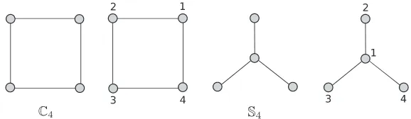
Fig. 1.4 Two unlabelled graphs, namely the cycleC4and the star graphS4, and one possible labelling of such two graphs.this case, no label is attached to the nodes, and the graph itself is said to beunlabelled. Figure 1.4 shows two examples of unlabelled graphs with N = 4 nodes, namely the cycle, usually indicated as C4, and the star graph with a central node and three links, S4, and two possible labellings of their nodes. Since the same unlabelled graph can be
represented in several different ways, how can we state that all these representations cor-respond to the same graph? By definition, two unlabelled graphs are the same if it is possible to label them in such a way that they are the same labelled graph. In particu-lar, if two labelled graphs are isomorphic, then the corresponding unlabelled graphs are the same.
It is easy to establish whether two labelled graphs with the same number of nodes and edges are the same, since it is sufficient to compare the ordered pairs that define their edges. However, it is difficult to check whether two unlabelled graphs are isomorphic, because there areN! possible ways to label theNnodes of a graph. In graph theory this is known as theisomorphism problem, and to date, there are no known algorithms to check if two generic graphs are isomorphic in polynomial time.
Another definition which has to do with the permutation of the nodes of a graph, and is useful to characterise its symmetry, is that of graphautomorphism.
Definition 1.3 (Automorphism)
Given a graph G = (N,L), an automorphism of G is a permutationφ :N →N of the vertices of G so that if(u,v)∈ Lthen(φ(u),φ(v))∈L.The number of different automorphisms of G is denoted as aG.
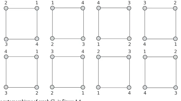
In other words, an automorphism is an isomorphism of a graph on itself. Consider the first labelled graph in Figure 1.4. The simplest automorphism is the one that keeps the node labels unchanged and produces the same labelled graph, shown as the first graph in Figure 1.5. Another example of automorphism is given byφ(1)=4,φ(2)=1,φ(3)=2, φ(4)=3. Note that this automorphism can be compactly represented by the permutation (1, 2, 3, 4) → (4, 1, 2, 3). The action of such automorphism would produce the second graph shown in Figure 1.5. There are eight distinct permutations of the labels (1, 2, 3, 4) which change the first graph into an isomorphic one. The graphC4has thereforeaC4 =8. The figure shows all possible automorphisms. Note that the permutation (1, 2, 3, 4) →
t
Fig. 1.5 All possible automorphisms of graphC4in Figure 1.4.Example 1.3
Consider the star graphS4with a central node and three links shown in Figure1.4. There are six automorphisms, corresponding to the following transformations: identity, rotation by 120◦counterclockwise, rotation by 120◦clockwise and three specular reflec-tions, respectively around edge (1, 2), (1, 3), (1, 4). There are no more automorphisms, because in all permutations, node 1 has to remain fixed. Therefore, the numberaGof
pos-sible automorphisms is given by the number of permutations of the three remaining labels, that is, 3!=6.
Finally, we consider some basic operations to produce new graphs from old ones, for instance, by merging together two graphs or by considering only a portion of a given graph. Let us start by introducing the definition of theunionof two graphs. LetG1 = (N1,L1)
andG2=(N2,L2) be two graphs. We define graphG=(N,L), whereN =N1∪N2and
L =L1∪L2, as theunionofG1andG2, and we denote it asG =G1+G2. A concept
that will be very useful in the following is that ofsubgraphof a given graph.
Definition 1.4 (Subgraph)
Asubgraphof G = (N,L)is a graph G′ = (N′,L′)such thatN′ ⊆N andL′ ⊆L. If G′ contains all links of G that join two nodes inN′, then G′is
said to be thesubgraph inducedorgeneratedbyN′, and is denoted as G′=G[N′].
Figure 1.6 shows some examples of subgraphs. A subgraph is said to bemaximalwith respect to a given property if it cannot be extended without losing that property. For example, the subgraph induced by nodes 2, 3, 4, 6 in Figure 1.6 is the maximal complete subgraph of order four of graphG. Of particular relevance for some of the definitions given in the following is the subgraph of the neighboursof a given nodei, denoted asGi.Giis
defined as the subgraph induced byNi, the set of nodes adjacent toi, i.e.Gi =G[Ni]. In Figure 1.6, graph (c) represents the graphG6, induced by the neighbours of node 6.
t
Fig. 1.6 A graphGwithN=6 nodes (a), and three subgraphs of G, namely an unconnected subgraph obtained by eliminating four of the edges ofG(b), the subgraph generated by the setN6= {1, 2, 3, 4, 5}(c), and a spanning tree (d) (one of the connected subgraphs which contain all the nodes of the original graph and have the smallest number of links, i.e.K=5).G′ =(N,L−L′), or simplyG′ =G−L′, the new graph obtained fromGby removing
all edgesL′.
1.2 Directed, Weighted and Bipartite Graphs
Sometimes, the precise order of the two nodes connected by a link is important, as in the case of the following example of the shuttles running between the terminals of an airport.
Example 1.4
(Airport shuttle) A large airport has six terminals, denoted by the lettersA,B,C,D,EandF. The terminals are connected by a shuttle, which runs in a circular path,
where theN =6 nodes represent the terminals, while the links indicate the presence of a shuttle connecting one terminal to another. Notice, however, that in this case it is neces-sary to associate a direction with each link. A directed link is usually called an arc. The graph shown in the right-hand side of the figure has indeedK =8 arcs. Notice that there can be two arcs between the same pair of nodes. For instance, arc (A,D) is different from arc (D,A).
We lose important information if we represent the system in the example as a graph accord-ing to Definition 1.1. We need therefore to extend the mathematical concept of graph, to make it better suited to describe real situations. We introduce the following definition of thedirected graph.
Definition 1.5 (Directed graph)
A directed graph G≡(N,L)consists of two sets,N = ∅ andL. The elements ofN ≡ {n1,n2,. . .,nN}are the nodes of the graph G. The elements ofL≡ {l1,l2,. . .,lK}are distinct ordered pairs of distinct elements ofN, and are calleddirected links, or arcs.
In a directed graph, an arc between nodeiand nodej is denoted by the ordered pair (i,j), and we say that the link is ingoinginjandoutgoingfromi. Such an arc may still be denoted aslij. However, at variance with undirected graphs, this time the order of the two
nodes is important. Namely,lij≡(i,j) stands for an arc fromitoj, andlij=lji, or in other
terms the arc (i,j) is different from the arc (j,i).
Box 1.2 DATA SET 1: Elisa’s Kindergarten Network
Elisa’s kindergarten network describesN = 16children between three and five years old, and their declared friendship relations. The network given in this data set is a directed graph withK=57arcs and is shown in the figure. The nine girls are represented as circles, while the seven boys are squares. Bidirectional relations are indicated as full-line double arrows, while purely unidirectional ones as dashed-line arrows. Notice that only a certain percentage of the relations are reciprocated.
It is interesting to notice that, with the exception of Elvis, the youngest boy in the class, there is almost a split between two groups, the boys and the girls. You certainly would not observe this in a network of friendship in a high school. In the kindergarten network, Matteo is the child connecting the two communities.
Summing up, the most basic definition is that of undirected graph, which describes systems in which the links have no directionality. In the case, instead, in which the directionality of the connections is important, the directed graph definition is more appro-priate. Examples of an undirected graph and of a directed graph, withN =7 nodes, and
K=8 links andK=11 arcs respectively, are shown in Figure 1.7 (a) and (b). The directed graph in panel (b) does not contain loops, nor multiple arcs, since these elements are not allowed by the standard definition of directed graph given above. Directed graphs with either of these elements are calleddirected multigraphs[48, 47, 308].
Also, we often need to deal with networks displaying a large heterogeneity in the rel-evance of the connections. Typical examples are social systems where it is possible to measure the strength of the interactions between individuals, or cases such as the one discussed in the following example.
t
Fig. 1.7 An undirected (a), a directed (b), and a weighted undirected (c) graph withN=7 nodes. In the directed graph, adjacent nodes are connected by arrows, indicating the direction of each arc. In the weighted graph, the links with different weights are represented by lines with thickness proportional to the weight.set of connecting roads that has minimum cost? It is clear that in determining the best construction strategy one should take into account the construction cost of the hypothetical road connecting directly each pair of towns, and that the cost will be roughly proportional to the length of the road.
All such systems are better described in terms ofweighted graphs, i.e. graphs in which a numerical value is associated with each link. The edge values might represent the strength of social connections or the cost of a link. For instance, the systems of towns and roads in Example 1.5 can be mapped into a graph whose nodes are the towns, and the edges are roads connecting them. In this particular example, the nodes are assigned a location in space and it is natural to assume that the weight of an edge is proportional to the length of the corresponding road. We will come back to similar examples when we discussspatial graphs in Section 8.3. Weighted graphs are usually drawn as in Figure 1.7 (c), with the links with different weights being represented by lines with thickness proportional to the weight. We will present a detailed study of weighted graphs in Chapter 10. We only observe here that a multigraph can be represented by a weighted graph with integer weights.
Finally, abipartite graphis a graph whose nodes can be divided into two disjoint sets, such that every edge connects a vertex in one set to a vertex in the other set, while there are no links connecting two nodes in the same set.
Definition 1.6 (Bipartite graph)
A bipartite graph, G≡(N,V,L), consists of three sets,N = ∅,V = ∅andL. The elements ofN ≡ {n1,n2,. . .,nN}andV ≡ {v1,v2,. . .,vV} are distinct and are called the nodes of the bipartite graph. The elements of L ≡ {l1,l2,. . .,lK}are distinct unordered pairs of elements, one fromN and one fromV, and are calledlinksoredges.
Many real systems are naturally bipartite. For instance, typical bipartite networks are systems of users purchasing items such as books, or watching movies. An example is shown in Figure 1.8, where we have denoted the user-set asU = {u1,u2,· · ·,uN}and
the object-set asO= {o1,o2,· · ·,oV}. In such a case we have indeed only links between
t
Fig. 1.8 Illustration of a bipartite network ofN=8 users andV=5 objects (a), as well as its user-projection (b) and object-projection (c). The link weights in (b) and (c) are set as the numbers of common objects and users, respectively.Box 1.3 Recommendation Systems
Consider a system of users buying books or selecting other items, similar to the one shown Figure 1.8. A reasonable assumption is that the users buy or select objects they like. Based on this, it is possible to construct
recommendation systems, i.e. to predict the user’s opinion on those objects not yet collected, and eventually to recommend some of them. The simplest recommendation system, known asglobal ranking method(GRM), sorts all the objects in descending order of degree and recommends those with the highest degrees. Such a recommendation is based on the assumption that the most-selected items are the most interesting for the average user. Despite the lack of personalisation, the GRM is widely used since it is simple to evaluate even for large networks. For example, the well-knownAmazon List of Top SellersandYahoo Top 100 MTVs, as well as the list of most downloaded articles in many scientific journals, can all be considered as results of GRM. A more refined recommendation algorithm, known ascollaborative filtering (CF), is based on similarities between users and is discussed in Example 1.13 in Section 1.6, and in Problem 1.6(c).
starting from a bipartite network, we can derive at least two other graphs. The first graph is a projection of the bipartite graph on the first set of nodes: the nodes are the users and two users are linked if they have at least one object in common. We can also assign a weight to the link equal to the number of objects in common; see panel (b) in the figure. In such a way, the weight can be interpreted as a similarity between the two users. Analogously, we can construct a graph of similarities between different objects by projecting the bipartite graph on the set of objects; see panel (c) in the figure.
1.3 Basic Definitions
Definition 1.7 (Node degree)
Thedegreeki of a node i is the number of edges incident in the node. If the graph is directed, the degree of the node has two components: the number of outgoing links kouti , referred to as theout-degreeof the node, and the number of ingoing links kini , referred to as the in-degreeof node i. The total degree of the node is then defined as ki=kouti +kiin.In an undirected graph the list of the node degrees{k1,k2,. . .,kN}is called thedegree sequence. The average degreekof a graph is defined ask =N−1N
i=1ki, and is equal
to k = 2K/N. If the graph is directed, the degree of the node has two components: the average in- and out-degrees are respectively defined askout = N−1N
i=1kouti and kin =N−1N
i=1kiin, and are equal.
Example 1.6
(Node degrees in Elisa’s kindergarten) Matteo and Agnese are the two nodes with the largest in-degree (kin = 7) in the kindergarten friendship network intro-duced in Box 1.2. They both have out-degreeskout=5. Gianluca has the smallest in and out degree,kout=kin=1. The graph average degree iskout = kin =3.6Another central concept in graph theory is that of the reachability of two different nodes of a graph. In fact, two nodes that are not adjacent may nevertheless be reachable from one to the other. Following is a list of the different ways we can explore a graph to visit its nodes and links.
Definition 1.8 (Walks, trails, paths and geodesics)
A walk W(x,y) from node x tonode y is an alternating sequence of nodes and edges (or arcs) W = (x ≡
n0,e1,n1,e2,. . .,el,nl≡ y)that begins with x and ends with y, such that ei=(ni−1,ni) for i=1, 2,. . .,l. Usually a walk is indicated by giving only the sequence of traversed nodes: W = (x ≡ n0,n1, ..,nl ≡ y). The length of the walk, l = ℓ(W), is defined as the number of edges (arcs) in the sequence. Atrailis a walk in which no edge (arc) is repeated. Apathis a walk in which no node is visited more than once. Ashortest path
(or geodesic) from node x to node y is a walk of minimal length from x to y, and in the following will be denoted asP(x,y).
Basically, the definitions given above are valid both for undirected and for directed graphs, with the only difference that, in an undirected graph, if a sequence of nodes is a walk, a trail or a path, then also the inverse sequence of nodes is respectively a walk, a trail or a path, since the links have no direction. Conversely, in a directed graph there might be a directed path fromxtoy, but no directed path fromytox.
Based on the above definitions of shortest paths, we can introduce the concept of
distancein a graph.