Graph, networks and design

Stochastic Geometry and Random Graphs for the

Analysis and Design of Wireless Networks

Martin Haenggi,

Senior Member, IEEE

, Jeffrey G. Andrews,

Senior Member, IEEE

, Franc¸ois Baccelli,

Olivier Dousse,

Member, IEEE

, and Massimo Franceschetti,

Member, IEEE

(Invited Paper)

Abstract—Wireless networks are fundamentally limited by the intensity of the received signals and by their interference. Since both of these quantities depend on the spatial location of the nodes, mathematical techniques have been developed in the last decade to provide communication-theoretic results accounting for the network’s geometrical configuration. Often, the location of the nodes in the network can be modeled as random, following for example a Poisson point process. In this case, different techniques based onstochastic geometryand thetheory of random geometric graphs – including point process theory, percolation theory, and probabilistic combinatorics – have led to results on the connectivity, the capacity, the outage probability, and other fundamental limits of wireless networks. This tutorial article surveys some of these techniques, discusses their application to model wireless networks, and presents some of the main results that have appeared in the literature. It also serves as an introduction to the field for the other papers in this special issue.

Index Terms—Tutorial, wireless networks, stochastic geometry, random geometric graphs, interference, percolation

I. INTRODUCTION

Emerging classes of large wireless systems such as ad hoc and sensor networks and cellular networks with multihop cov-erage extensions have been the subject of intense investigation over the last decade. Classical methods of communication theory are generally insufficient to analyze these new types of networks for the following reasons: (i) The performance-limiting metric is the signal-to-interference-plus-noise-ratio (SINR) rather than the signal-to-noise-ratio (SNR). (ii) The interference is a function of the network geometry on which the path loss and the fading characteristics are dependent upon. (iii) The amount of uncertainty present in large wireless networks far exceeds the one present in point-to-point systems: it is impossible for each node to know or predict the locations and channels of all but perhaps a few other nodes.

Two main tools have recently proved most helpful in cir-cumventing the above difficulties: stochastic geometry [1] and random geometric graphs [2], [3]. Stochastic geometry allows to study the average behavior over many spatial realizations of a network whose nodes are placed according to some probability distribution. Random geometric graphs capture the distance-dependence and randomness in the connectivity of the nodes. This paper provides an introduction to these mathematical tools and discusses some recent results that were enabled by them, with the objective of being a first-hand tutorial for the researcher interested in the field.

A. The role of the geometry and the interference

Since Shannon’s work [4], for the second half of the 20th century the SNR has been the main quantity of interest to communication engineers that determined the reliability and the maximum throughput that could be achieved in a communication system. In a wireless system, the SNR can vary among different users by as much as ten to hundreds of dBs due to differences in path loss, shadowing due to buildings and obstructions, fading due to constructive or destructive wave interference. The first-order contributor to this SNR variation is the path loss. In a cellular system for example, it is not uncommon for a user close to the base station to have a channel that is a million times (60 dB) stronger than the one of a user located near the cell’s edge. If the receivers are randomly located in space, then the different SNRs due to the different path losses between them and the base station can be modeled as having aspatialdistribution.

In a wireless network with many concurrent transmissions, the situation is even more complicated. In this case, the SINR becomes the relevant figure of merit for the system1. Not only the received signal power is random due to the random spatial distribution of the users, but also the interference power is governed by a number of stochastic processes including the random spatial distribution of the nodes, shadowing, and fading. The SINR for a receiver placed at the origin oin the

2 or3-dimensional Euclidean space can be written as:

SINR₌ S

W +I, where I= X

i∈T

Pihiℓ(kxik), (1)

whereS, W, andI are the desired signal, noise, and interfer-ence powers, respectively. The summation forI is taken over the set of all interfering transmitters _T, Pi is the transmit

power, hi is a random variable that characterizes the

cumu-lative effect of shadowing and fading, andℓ is the path loss function, assumed to depend only on the distance_kxik from

the origin of the interferer situated at position xi in space.

Oftenℓis modeled as a power law,ℓ(kxik) =k0kxik−α, or in

environments where absorption is dominant, as an exponential law, ℓ(kxik) = k0exp(−γkxik), see [5], [6]. In a large

system, the unknowns are_T,hi, andxi, and perhapsPi, but it

is the locations of the interfering nodes that most influence the SINR levels, and hence, the performance of the network. The

1_{In many practical situations such as cellular networks and reasonably}

interference is a function of the underlying node distribution (and mobility pattern for mobile networks) and the channel access scheme.

A key objective of this tutorial and special issue is to show that the SINR in (1) can be characterized using stochastic techniques, and key related metrics such as outage probability, coverage, connectivity, and capacity can therefore be quanti-fied.

B. Historical background

Although there has been growing recent interest in the use of stochastic geometry and random graph theory to describe wireless networks, some of the underlying approaches go back 100 years, or more. Wireless network performance is mostly interference-limited, and a large number of users contribute to the interference in vastly varying magnitudes, as described by the interference function stated in (1), which is a shot noise process. In one dimension, a shot noise process is defined as

I(x) =

∞

X

i=−∞

g(x₋Xi), (2)

where_{Xi}is a stationary Poisson process on Randg(x)is

the impulse response of a linear system. In its two-dimensional generalization, x represents a point on the plane and the Poisson point process is on R2_{. Wheng(x) depends only on} the Euclidean norm kxk, it can be identified with the path loss function ℓ(kxk), and I(x) is the aggregate interference received at point x in a wireless network, without fading. The shot noise process has been studied at least dating back to Campbell in 1909 [7], who characterized its mean and variance, followed by Schottky in 1918 [8]. In addition, Rice performed extensive investigations on the distribution ofI(x)

from 1940 through 1970 [9]. Power law shot noise – most relevant here – was considered by Lowen and Teich in 1990 [10].

Stochastic geometry has been used as a tool for characteriz-ing interference in wireless networks at least as early as 1978 [11], and was further advanced by Sousa and Silvester in the early 1990s [12]–[14]. At that time, two useful mathematics texts were available to researchers: Stoyan et al.’s stochastic geometry first edition in 1987 (see [1] for the second edition) and Kingman’s Poisson Processes [15]. In the late 1990’s, Ilow and Hatzinakos [16] characterized the impact of random channel effects – fading, shadowing, path loss, and combina-tions thereof – on the aggregate co-channel interference, while Baccelli et al. also began developing tools primarily based on Poisson Voronoi tesselations and Delaunay triangulations for the optimization of hierarchical networks [17], [18] and of mobility management in cellular networks [19]. For a survey on this line of research, see the forthcoming book chapter by Zuyev [20].

In the past ten years, stochastic geometry and associated techniques have been applied and adapted to cellular systems [21]–[24], ultrawideband [25], cognitive radio [26]–[28], fem-tocells [29], [30], relay networks [31], and many other types of wireless systems. However, perhaps the largest impact has been in the area of ad hoc networks, which are fully distributed

and in which all participating nodes – both transmitters and receivers – are randomly located. In such networks, it is impossible even with unlimited overhead to control the SINRs of all users, due to the coupling of interference: if one user raises its power, it causes an interference increase to all other communicating pairs. In this case, characterizing the (stochastic) geometry of the network is of utmost importance since it is the first-order determinant of the SINR.

The idea of modeling wireless networks using random graphs dates back to Gilbert [32], whose paper marks the starting point for continuum percolation theory. He considered a random network formed by connecting points of a Poisson point process that are sufficiently close to each other. Using this model, he proved the existence of a critical connection distance above which an infinite chain of connected nodes forms and below which, in contrast, any connected component is bounded. His investigations were based on prior work on the discrete percolation model of Broadbent and Hammersley [33] and on the theory of branching processes [34]. Gilbert’s origi-nal model has undergone many generalizations, and continuum percolation theory is now a rich mathematical field, see [2], [35]. Extensions most relevant to us consider graphs which account for interference-limited communication. In this case, the graph connectivity depends on the SINR at different nodes. These are studied in [36] and [37]. Another relevant generalization is the random connection model [38], which is a random graph that can account for random connections due to shadow fading effects; as well as nearest neighbor network models [39]. Finally, a coverage model for wireless networks based on percolation theory was introduced in [40]. A compendium of random graph results related to wireless communications appears in [3]. Elements of random graphs have also proven to be useful to characterize the scaling behavior of the capacity of wireless networks [41].

C. Paper overview and organization

In §II, we provide an overview of the key mathematical tools, including point processes, random geometric graphs, and percolation. In_§III, the interference is characterized, and it is shown that the outage probability is a natural metric to study in a spatially random wireless network. We then move to other performance metrics, such as the connectivity of the network and its coverage in _§IV, and the data-carrying capacity and area spectral efficiency of the network in _§V. We conclude by providing some additional applications of these results, including epidemic models, wireless security, and transmission protocol design. The notation and symbols used in the paper are listed in Table I.

II. MATHEMATICALPRELIMINARIES

Symbol Definition/explanation [k] the set{1,2, . . . , k}

Z,N integers, positive integers

R,R+ _{real numbers, positive real numbers}

1A(x) indicator function

u(x) ,1{x>0}(x)(unit step function)

d number of dimensions of the network #A cardinality ofA

P_(A) probability of eventA

E(X) expectation of random variableX

LX(s) =E(e−sX) Laplace transform of random variableX

| · | Lebesgue measure

k · k Euclidean norm

o origin inRd

B a Borel subset ofRorRd

B(x;r) ball of radiusrcentered atx cd ,πd/2/Γ(1 +d/2)

(volume of thed-dim. unit ball)

α path loss exponent

FX(x) =P(X6x) distribution of random variableX(cdf)

Φ ={Xi} ⊂Rd point process

Λ, λ counting measure and density forΦ

pc, λc critical probability, density for percolation

h (power) fading random variable (E(h) = 1)

T∈R+ SIR or SINR threshold for successful communication

ǫ∈(0,1) target outage probability for transmission capacity

ℓ:R_→R+ (isotropic) large-scale path loss function

W thermal noise

TABLE I

NOTATION AND SYMBOLS USED IN THE PAPER.

A. Point processes

The most basic objects studied in stochastic geometry are point processes. Visually, a point process can be depicted as a random collection of points in space. More formally, a point process (PP) is a measurable mapping Φ from some probability space to the space of point measures (a point measure is a measure which is locally finite and which takes only integer values) on some spaceE. Each such measure can be represented as a discrete sum of Dirac measures onE:

Φ =X

i

δXi.

The random variables_{Xi}, which take their values inE are

the points of Φ. Most often, the space E is the Euclidean space Rd _{of dimension d ≥ 1. The intensity measure Λ of}

Φ is defined as Λ(B) = E_{Φ(B) for Borel B, where Φ(B)} denotes the number of points in Φ∩B.

A few dichotomies concerning point processes on Euclidean space Rd _{are as follows:}

• A PP can be simple or not. It is simple if the multiplicity of a point is at most one (no two points are at the same location).

• A PP can be stationary or not. Stationarity holds if the law of the point process is invariant by translation.

• A PP can be Poisson or not. A formal definition of the Poisson point process (PPP) is given in the following sub-section. A PPP offers a handy computational framework for different network quantities of interest.

– A PPP can be homogeneous or not. In the homo-geneous case, the density of the points is constant across space.

– The homogeneous PPP is stationary and simple. This may be considered as the simplest (and most natural) point process.

– The framework for non-homogeneous PPPs is also well developed, although more technical than that of the homogeneous case. They can be used to model distributions of users which are not uniform across space.

– There is also a comprehensive computational frame-work for stationary point processes which are not Poisson. This is Palm calculus (see below).

• A point process can beisotropicor not. Isotropy holds if the law of the PP is invariant to rotation. The homoge-neous PPP is isotropic. If a PP is isotropic and stationary, it is called motion-invariant.

• A PP can be marked or not; marks assign labels to the points of the process, and they are typically independent of the PP and i.i.d. The study of marked point processes may require the handling of Palm calculus.

1) Poisson point processes: Let Λbe a locally finite mea-sure on some metric spaceE. A point processesΦis Poisson onE if

• For all disjoint subsets A1,· · ·, An of E, the random

variablesΦ(Ai) are independent;

• For all sets A of E, the random variables Φ(A) are Poisson.

A key property states that conditionally on the fact that

Φ(A) =n, these n points are independently (and uniformly for homogeneous PPP) located inA. This leads to an explicit representation of the Laplace functional ofΦ. IfE=Rd_{, this} Laplace functional is defined for general point processesΦby

LΦ(f),E h

e−RRdf(x) Φ(dx)

i

=Eh_e−PX∈Φf(X) i

,

wheref is a non-negative function onRd_{. In the Poisson case,}

LΦ(f) = exp

− Z

Rd

1₋e−f(x)_Λ(dx)

. (3)

This is the basis for a large number of formulas like,e.g., those on the Laplace transform of the shot noise (or interference), see_§III. Other appealing features of PPPs are their invariance to a large number of key operations. In particular,

• The superposition of two or more independent PPPs (which is defined as the sum of the associated point measures) is again a PPP; this can be extended to denumerable sums under some conditions.

• The independent thinning of a PPP is again a PPP; this can be extended to the case of location-dependent thinning, where a point is retained or not depending on its location.

• The point process obtained by displacing pointXi

inde-pendently of everything else according to some Markov kernel K(Xi,·) that defines the distribution of the

dis-placed position of the pointXi yields another PPP; this

If ρ(x,_·) is the probability density pertaining to the Markov kernel applied to a PPP of intensityλ(x)onRd_{, the displaced} points form a PPP of intensity

λ′(y) =

Z

Rd

λ(x)ρ(x, y)dx .

In particular, if λ(x) is constant λand ρ(x, y) is a function ofy−xonly, then λ′(y) =λfor ally.

A striking property of PPPs is Slivnyak’s theorem which states that the law ofΦ₋δxconditional on the fact thatΦhas

a point atxis the same as the law ofΦ. In mathematical terms, the reduced Palm probability Px! _{of a PPP is the distribution} of this Poisson point process itself. This is usually expressed as Px!_{=P, for all pointsx∈Φ. This means that the properties} seen from a pointx∈Rd _{are the same whether we condition} on having a point x∈ Φ or not — if the point at x is not considered. For example, we have for the mean number of points within distance rofx:

E_{Φ(B(x;r)\ {x}) =} E_{Φ(B(x;r)\ {x}) | x∈Φ}

= Λ(B(x;r)),

whereB(x;r)is the ball of radiusr centered atx.

2) Stationary point processes: The theory of stationary point processes is based on the concept of marks and on the Matthes definition of Palm probability [42], [43].

Roughly speaking, a mark of some point of a stationary point process is a quantity that “follows this point” when the collection of points is transported by a global translation operation. For instance, the local configuration of neighbors of point X, which is defined as the collection of points in a ball of radiusR centered atX, is a mark of this point. IfR is infinity, this mark is the universal mark of X, namely ’the point process seen from X’.

The Palm probability Po _{of a stationary point process is}

the law of this universal mark, which can be shown to be the same for all points. It can be understood as the law of the point process given that it has a point at the origin. As defined here Po _{is a probability on the space of point measures.}

Campbell’s formula for stationary point processes, which is a direct consequence of the last definition, states that when denoting byΦ₋xthe global translation of all points ofΦby the vectorx, then

E

" X

X∈Φ

f(X,Φ₋X)

#

=

Z

N

Z

Rd

f(x, φ)λdxPo(dφ), (4)

where _N is the space of simple point sequences, for all positive functions f(x, φ) ofx_∈Rd _{andφ a point measure} on Rd_{. Hereλis the intensity ofΦ, that is the mean number} of points per unit space. The last formula is the key tool for computing the mean values of sums on the points of a stationary point process. Applied to PPPs, they are particularly simple. Let Φbe a stationary PPP of intensityλonRd_{. Then} for non-negativef,

E X

X∈Φ f(X)

!

=λ Z

Rd

f(x)dx (5) and

var X

X∈Φ f(X)

!

=λ Z

Rd

f2(x)dx . (6)

These expressions can be used, for example, to calculate the mean and variance of the interference in a network or to determine the mean node degree.

Important examples of stationary point processes that lead to nice computational results include

• point processes with repulsion, e.g., Mat´ern hard core point processes or determinantal point processes;

• point processes with attraction,e.g., Neyman-Scott cluster processes, permanental point processes [44] or Hawkes point processes [45].

For more on this, see [1] and [42].

B. Boolean models and random geometric graphs

1) The germ–grain model: The most celebrated model of stochastic geometry and the basic model of continuum per-colation is the Boolean or germ-grain model. In the simplest setting, the Boolean model is based on a Poisson point process

Φ, the points of which,_{Xi}, are also calledgerms, and on an

independent sequence of i.i.d. compact sets _{Ki} called the grains. Formally, the Boolean model is

Ξ =[ i

(Xi+Ki)

whereXi+Ki={Xi+y, y∈Ki}.

The Poisson set of germs and the independence of the grains make the Boolean model analytically tractable. It is often considered as the null hypothesis in stochastic geometry modeling.

Among the key results on this model, let us quote (from [1]):

• Coverage: the simplest coverage question is the distri-bution of the number of grains that intersect a given compact set, for instance a given location of the space. This distribution is Poisson.

• Volume fraction: in the homogeneous case, what is the fraction of a big ball which is covered by grains? This can be derived using the analysis of coverage and an ergodic theorem.

• Contact distribution: given that a location is not covered,

what is the radius of the bigest ball (resp. length of the longest segment of orientationθ) centered at this location that does not intersect any grain of the Boolean model?

2) Gilbert’s random disk graph: This is a model for wire-less networks that is a special case of the Boolean model described above, and is due to Gilbert [32]. Assume that the compact sets described in the last subsection are all balls of radiusr/2. We define the random disk graph of a Poisson point

Φprocess of intensityλwith ranger, denoted as Gλ,r as the

graph with nodes the points ofΦ and with edges betweenX and Y if the two grains touch,i.e., if _kX₋Y_{k ≤}r. This is the most basic random geometric graph and a central object in random graph theory. The following questions are of particular interest within this setting:

• Does this random graph has an infinite component? This is of course equivalent toΞhaving an infinite component. This property is referred to as percolation. A striking result is that there is a deterministic critical value 0 < rc <∞such that whenr < rc, there is no such infinite

component with probability 1 (i.e., there is no percolation for all realizations ofΦ), whereas when r > rc, there is

an infinite component with probability 1 (i.e., there is percolation for all realizations of Φ). This is proven in §IV-C.

• In case percolation occurs, what is the fraction of nodes included in the infinite component? In case of it does not occurr, what is the typical size of a component? The main tool for addressing these continuum percolation questions is a reduction to discrete bond or site percolation. For more on the matter, see [3], [35], [47].

C. Voronoi tessellation

By definition, a tessellation is a collection of open, pairwise disjoint polyhedra (polygons in the case ofR2_{) whose closures} cover the space, and which is locally finite (i.e., the number of polyhedra intersecting any given compact set is finite).

Given a simple point measure (or point sequence)φonRd and a point x∈Rd_{, we define theVoronoi cellCx(φ) of the} pointx∈Rd _{w.r.t. φto be the set}

Cx(φ) ={y∈Rd:ky−xk< inf xi∈φ,xi6=xk

y−xik}. (7)

For a simple point process Φ = P

iδXi on R

d_{, we define}

the Voronoi tessellation ormosaic generated by Φ to be the marked point process

V=X i

δ(Xi,C_Xi(Φ)−Xi),

whose marks are the Voronoi cells shifted to the origin. The Delaunay triangulation generated by a simple point measure φ is a graph with the set of vertices φ and edges connecting each y_∈φto any of its Voronoi neighbors.

The Delaunay triangulation of a Poisson point process is an object of central importance in communications. In a regular periodic (say hexagonal or triangular) grid it is obvious how to define the neighbors of a given vertex. However, for irregular patterns of points like a realization of a PPP, which is often used to model set of nodes in mobile ad hoc networks, this notion is much less evident. The Delaunay triangulation offers some purely geometric definition of neighborhood in such patterns.

For quantitative properties of Poisson–Voronoi tessellations (mean cell size, mean number of sides of the cell, etc.) and Poisson–Delaunay graphs (mean degree, mean length of a typical edge, mean size of a typical triangle) see, e.g., [48]. In [17], [18], [49], Voronoi tessellation-based models of cellular access network were considered to derive closed-form expressions for the mean number of users in a cell, the mean length of connections, and the total power received at the base station.

III. INTERFERENCECHARACTERIZATION ANDOUTAGE

In this section we apply some of the techniques introduced above to study the interference in large ad hoc networks and the outage probability of any given link.

A. Interference

We start with the general question: what can be said of the total interference power measured at a pointxin the network, given by

I(x), X

Y∈Φt

ℓ(_kx₋Y_k),

where Φt is a point process of transmitters (assumed to be

interferers) on R2_{?Φt is typically a subset of a larger point} processΦsince it constitutes the nodes selected by the MAC scheme to transmit concurrently. For example, if nodes in a homogeneous PPP of intensity 1 transmit independently and randomly with probability p (slotted ALOHA), Φt is a PPP

with intensity p. Due to Slivnyak’s result (see §II-A1), I(x)

does not depend on the given location where interference is measured; in particular, it does not matter whether x is part of the underlying point process Φ or not (as long as its contribution to I is not considered if Φt is conditioned on

having a point atx).

As mentioned in§I-B, researchers have followed an analogy toshot noise processesto analyze the distributional properties ofI(x)[9], [16], [50]. This analogy can be used to derive the Laplace transform of the interference as follows.

Let Φ , _{Ri = kXik} be the distances of the points

of a d-dimensional uniform PPP of intensity µ from an arbitrary origin o. Then Φ is an inhomogeneous PPP with intensity function λ(r) = µcddrd−1, where cd = |B(o,1)|

is the volume of thed-dimensional unit ball. Considering the interference as a shot noise process (2), and also accounting for the fading terms, we can identifyhrℓ(r) =hrr−αfor i.i.d.

fadinghwith the impulse response of the shot noise process. We would then like to calculate the Laplace transform

LI(s),E[e−sI] =E

" Y

R∈Φ

exp ₋shRR−α

#

of the interference. This is a Laplace functional with f(r) =

product, so we have from (3) (see also [61, Eqn. (3)])

LI(s) = exp

−

Z ∞ 0

E_h[1−e−shr−α_]λ(r)dr

= exp₋µcdE[hδ]Γ(1−δ)sδ

, (8)

where δ , d/α. Note that this expression is only valid for δ <1. So:

• Forα6d, we haveI=_∞a.s. This is a consequence of the cumulated interference from the many far transmitters whose signal powers do not decay fast enough to keep the interference power finite. For a finite network, the interference would be finite.

• Forα > dwe haveI <∞a.s. butE_{(I) =∞due to the} singularity of the path loss law at the origin. Even if we consider only the nearest interferer, E_{(I)is infinite. If a} bounded path loss law is used, all moments exist. In the important case of Rayleigh fading,E_[hδ_{] = Γ(1 +δ),} so, using the properties of the gamma function, we obtain the closed-form result

LI(s) = exp

−µcdsδ

πδ

sin(πδ)

.

So the interference has astable distributionwith character-istic exponentδand dispersionµcdE[hδ]Γ(1−δ). Sinceδ <1,

I does not have any finite moments.

A closed-form expression for the interference distribution only exists for δ= 1/2; this is the inverse Gaussian or L´evy distribution, as has been established in [51].

Using the distribution of the distances to the n-th nearest neighbor [52], the distributions of the interference (without fading) from the n-th nearest neighbor are easily found. The tail probabilities do not depend on the presence or type of fading and are given by

P_{(In> x)∼} 1 n!(λcd)

n_x−nδ_{, x}

→ ∞.

This means that E_(Inp_{) exists for p < nδ. For example, if} interference-canceling techniques are used and the interference from theknearest interferers can be cancelled, we needk > α in two-dimensional networks to have a finite second moment. If the non-singular path loss model ℓ(x) = (1 +_kx_k)−α

is used, the tail probability of the interference reflects the tail probability of the fading process: If the fading has an expo-nential or power-law tail, so does the interference. This holds for general motion-invariant processes [53]. Other approaches to the singularity issue are given in this issue [54], [55].

B. Outage

Anoutageof a wireless link is said to occur when a packet transmission fails. In many situations, it is justified to equate the outage event to the event thatSINR_{< T for some threshold}

T that depends on the physical layer parameters such as rate of transmission, modulation, and coding. The complementary probability is the success probability ps,P(SINR>T).

In the case where the desired signalSis subject to Rayleigh fading, we obtain for the success probability over a link of

distanceR

ps=P(S > T(W+I)) = exp

−T R

α_W

P

E_(e−T RαI_), (9) where P is the transmit power. The first term only depends on the noise (or SNR), while the second only depends on the interference (or SIR). Focusing on this interference term we notice that this is the Laplace transform of the interference evaluated at s = T Rα_{. So, in a d-dim. interference-limited}

network whose nodes are distributed as a uniform PPP of intensity λ with ALOHA channel access with probabilityp, the success probability is given by (8), replacingsbyT Rα_:

ps= exp

−λpcdRdE[hδ]Γ(1−δ)Tδ

(10)

Here we have used the fact that ALOHA channel access performs independent thinning of the PPP, which results in a PPP of lower intensity. The interferers’ channels may be subject to a different type of fading (or no fading), all that matters isE_[hδ_].

The equivalence of Laplace transforms and success proba-bilities has been pointed out in [56]–[58], and in [58] several generalizations can be found.

C. Throughput

The transmission success probability in the previous subsec-tion is derived assuming that the desired transmitter transmits while the received listens. To optimize the network parameters, such as the ALOHA transmit probabilityp, the unconditioned success probabilities must be considered. In the case of ALOHA and half-duplex transceivers, thespatial throughput

is p(1−p)ps(p). Finding the optimum p means finding the

optimum trade-off between spatial reuse (a larger p results in a higher density of concurrent transmissions) and success probabilities (a largerpresults in higher interference and thus a lower success probability). In [58], a related metric, thespatial density of successppsis optimized in function ofp. In some

cases, the optimal value, which is known in closed form, does not depend on the intensityλof the underlying point process. The same framework can also be used to find the optimum value for the SINR thresholdT that maximizes thearea spec-tral efficiency. A larger T permits higher transmission rates (or spectral efficiencies if normalized by the bandwidth) but results in lower success probabilities (see further discussion in§V-B). Similarly, theprobabilistic progress, usually defined as the product of distance times success probability can be maximized by finding the optimum link distance R [59]. Choosing a larger R may increase the progress but comes with the disadvantage of a lower success probability [60]. In [58], an expression for progress based on extremal shot noise is derived, and in [61], the distribution and the mean value of the throughput of a typical user (as given by Shannon’s formula) are given using Fourier transform techniques.

IV. PERCOLATION ANDCONNECTIVITY A. Introduction

branch of probability. More recently, percolation models have been used to model the connectivity of wireless multi-hop networks.

The main property of percolation models is that they exhibit aphase transitionin their connectivity behavior: depending on some (continuous) parameters, the components of the model are either all finite (sub-criticalcase) or one giant component forms (super-criticalcase). In the context of networking, such a transition affects the performance of the system greatly: without a giant component, the network would be completely fragmented and unusable. It is therefore of prime importance to characterize the conditions under which the network is sucritical. In this section, we cover some basics of per-colation theory, starting with the simplest models and proof techniques, and then moving on to models that are more appropriate for wireless networks.

Percolation theory deals mostly with models of infinite size. We start with these classical models and briefly address finite networks.

B. Discrete percolation: Bond percolation in infinite lattices

The bond percolation model is defined as follows: consider the infinite square lattice Z2_{and connect each pair of nearest} neighbors independently with probability p. Then define the component (orcluster) of the originCas the set of elements of Z2 _{that are connected to the origin by a sequence of adjacent} edges. We define thepercolation probabilityas

θ(p) :=P_(#C=∞).

The central result of percolation theory is the following:

Theorem 1 (Broadbent and Hammersley [33]) There exists a number 0 < pc <1 such thatθ(p) = 0 forp < pc andθ(p)>0forp > pc.

In the particular case of bond percolation onZ2_{, the exact} value of pc is known to be1/2[62]. Other specific cases and

properties ofθ(p)can be found in [47]. To prove Theorem 1, we need first to observe that θ(p) is an increasing function. Although this is a very intuitive property, its proof is not so trivial (see,e.g., [35, Ch. 2.2] for a general method). It is then enough to prove that there exists some probability p1 > 0 such that θ(p1) = 0 and some probability p2 < 1 such that θ(p2)>0. The following two sections are devoted to finding p1 andp2.

1) Absence of percolation for small values of p: We start from the observation that if the origin belongs to an infinite cluster, then for any integer n, one can find in the lattice a self-avoiding path of length nstarting at the origin. Thus we have

θ(p)≤P_{(∃a path of lengthnstarting ato) ∀n . (11)}

If all direct neighbors of Z2 _{were connected by an edge, the} numberκ(n)of such path would be bounded from above by4_· 3n−1_{. Since edges are present with probabilityp, each of these} κpaths exists with probabilitypn_{. Using the union bound, we}

find that

P_{(∃a path of lengthn starting ato)≤4p(3p)}n−1_.

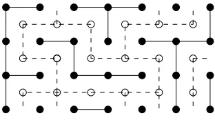
Fig. 1. A realization of the bond percolation model onZ2

(plain lines) and its dual (dotted lines).

If p < 1/3, this quantity tends to zero when n increases, so that (11) implies θ(p) = 0. So we have established that pc>1/3.

2) Existence of an infinite cluster for sufficiently large

p: Our proof relies on the classical Peierls argument [63]. Consider the dual lattice ofZ2_{, which consists of vertices that} are shifted by half a unit in both directions, as depicted in Figure 1. An edge is placed between two direct neighbors of the dual lattice if it does not intersect an edge of the direct lattice.

The key observation is that if a component is finite in the original lattice, it is necessarily surrounded by a circuit in the dual lattice. To prove that a vertex (e.g., the origin) belongs to an infinite cluster with positive probability, it is thus enough to show that the probability that a circuit surrounds the origin in the dual lattice is less than one. Let us estimate the number σ(n)of possible circuits of length2nthat surround the origin: it is easy to see that it is bounded by

σ(n)≤(n−1)·32(n−1).

Therefore, the probability that there exists a circuit around the origin with all edges closed upper bounded by

P_{(closed circuit) ≤}

∞

X

n=2

(1₋p)2nσ(n)

= 9(1−p)

4

[1−9(1−p)2_]2.

One can verify that when p > 1 −1/(2√3) ≈ 0.71, the above sum converges to a number smaller than one. As a consequence, the origin belongs to an infinite cluster with positive probability.

Note that since the existence of an infinite cluster does not depend on the state of a finite number of edges, we can use Kolmogorov’s zero-one law to conclude that the probability that such a cluster exists is either zero or one (seee.g., [64]). If it was zero, then the origin would belong to an infinite cluster also with probability zero. Therefore, wheneverθ(p)>0, an infinite cluster exists with probability one.

C. Continuum percolation: The random geometric graph

The basic random geometric graph or disk graph Gλ,r, as

from the following model: assume that nodes emit with a certain powerP and that this signal is attenuated over distance according to a deterministic decreasing functionℓ(d). Assume also that receivers can successfully receive data if the signal is at leastβ times stronger than the ambient noise, which has power W. Then the transmission radius is defined by

r,max{d: P ℓ(d)

W ≥β}. (12) Similarly to the discrete model, we denote by θ(λ, r) the probability that a node located at the origin belongs to an infinite cluster. Due to its simplicity, the graph Gλ,r can be

rescaled while keeping its connectivity properties. Indeed, if all distances are divided byγ, the underlying PPP is transformed into another Poisson process with intensity γ2_{λ. Thus, the} graph Gγ2_λ,r/γ has the same connectivity properties as G_λ,r and we have

θ(γ2λ, r/γ) =θ(λ, r).

As in the bond percolation model, we briefly explain a way to show that a phase transition occurs inGλ,r.

1) Absence of an infinite cluster for small values of λ:

Consider a nodeoplaced at the origin. We populate the setC of the nodes connected to ostep by step: at step zero, we set C=_{o_}. Then at each step, we add toCall nodes that share an edge with an element ofC. As each node has on average λπr2_{edges, this process can be compared to a Galton-Watson} process [34] where each individual gives birth toλπr2_children in average. The difference is that in our process, the number of nodes added at each step might be smaller, as some nodes sharing edges with elements ofCmight be already inC. It is known that if the average number of children per individual in a Galton-Watson process is smaller than one, the process stops after a finite number of steps [34]. As our process grows more slowly, it certainly stops in this case too. Therefore we have that ifλ <1/(πr2_{), the cluster of the origin is finite a.s.}

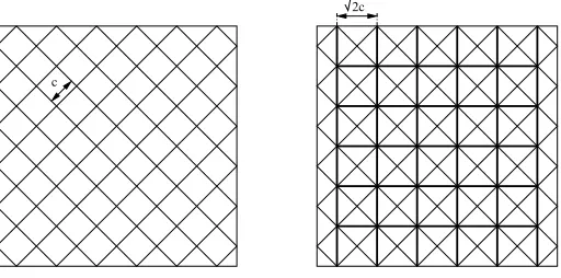
2) Existence of a giant cluster for large λ: We use a mapping onto a bond percolation model: We divide the plane into squares of size c =r/2√2 as shown in Figure 2. Each square corresponds to a potential edge of the lattice, which is added if at least one point of the Poisson process falls into this square. Thus, each edge is present with probability p = 1₋exp(₋λc2_{), independently of the other edges. As} a consequence, if λ _≥log 2/c2_{, the edge percolation model} contains an infinite cluster a.s.

Moreover, if two edges are adjacent, then by construction two points of the Poisson process are located in squares that share at least at one corner. Therefore, the distance between them is less than 2√2c = r, and they are connected in Gλ,r. Accordingly, an infinite collection of connected edges

corresponds to an infinite set of connected points in Gλ,r.

We can thus conclude that if λ≥log 2/c2_,G

λ,r contains an

infinite cluster a.s.

The exact value of the critical densityλc(r)or critical radius

rc(λ) is unknown. For λ = 1, the bounds 1.1979 < rc < 1.1988were established with 99.99%confidence in [65].

3) Generalization to the Boolean model: Gilbert’s random geometric graph is a particular case of the Boolean model (see §II-B). Let us consider a Boolean model of arbitrary dimension

2c

c

Fig. 2. On the left hand side, the division of the plane into squares. On the right hand side, each square is assigned to an edge of a bond percolation model (bold lines).

dwhere grains are balls whose radius is now random. It turns out that for a suitable radius distribution, a phase transition is observed at some critical germ density. Denoting byRthe (random) radius of a ball, one can show [35] that whenever the dimension of the modeldis greater than one andE_(R4_)<∞, there exists a critical value ofλbelow which the union of the balls Ξ has only finite components and above which a giant component forms.

D. Other models

In this section, we briefly describe other percolation models that are relevant to communication networks. In all of them, the location of the nodes is modeled by a Poisson point process of density λ over R2_{. They differ only by the criterion used} for adding edges between nodes.

1) Nearest-neighbors networks: In this model, each node connects to itsknearest neighbors. This model is for example suitable for a dense wireless network where nodes use power control algorithm in order to be connected only to theirkfirst neighbors.

An important property of this model is that the value of λ does not affect the connectivity of the model (it is called ascale-free model). Therefore, its only relevant parameter is k. One can show that there exists a critical value of k for which a giant component forms, and below which only finite clusters are observed. In two dimensions, the critical value is conjectured to bek= 3 [39].

2) Random connection model: This model is another gen-eralization of Gilbert’s model. For each pair of nodes, we consider the distancexbetween them. Then we add an edge between them with probability g(x), where g is a function fromR+ _{to[0,1]such that}R∞

0 xg(x)dx <∞.

density cannot increase. The spread-out limiting case has also been worked out in [67], showing that in the case of very long, unreliable connections, the critical density has a limit corresponding to that of an independent branching process, i.e. the average degree of the corresponding random graph at the percolation threshold tends to 1. Alternative proofs of these spreading results also appear in [68], [69].

3) Signal-to-interference ratio graph (STIRG) model: The connectivity criterion in (12) compares the received signal to the ambient noise only. However, if several nodes are using the same channel, interference degrades the received signals. In the so-called STIRG model [36], [37], the SNR threshold is replaced by an SINR threshold as in (9) so that the nodes Xi, Xj∈Φare connected by an edge if

P ℓ(kXi−Xjk)

W+γ(max_{I(Xi);I(Xj)} −P ℓ(kXi−Xjk)) ≥

T,

whereI(Xi) =P_Xk∈Φ\{Xi}P ℓ(kXi−Xkk). This condition

ensures that the two nodes have a sufficiently high SINR to exchange data in both directions despite the interference of all the other nodes. The factor γ≤1 serves as a weight for the interference term and models the gain of the spread spectrum scheme (if any).

This model differs from the others by the fact that if has more degrees of freedom. Clearly, when γ = 0, the model is equivalent to Gilbert’s model, and it percolates above the critical node density for Gilbert’s graph λc. In the case of

attenuation function of bounded support, it has been shown in [36] that for large enoughλone can chooseγsmall enough so that the model percolates. This result has been strengthened in [37] to show that this is the case whenever λ > λc and

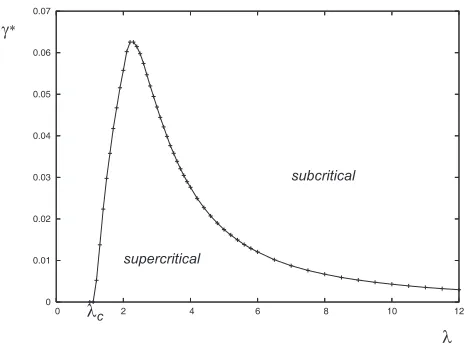
also for attenuation functions of unbounded support. In other words, whenever the node density is super-critical (in Gilbert’s sense), the model can tolerate a certain amount of interference before the giant component disappears. Figure 3 gives a picto-rial representation of this mathematical result obtained through computer simulation, illustrating the parameter domain where percolation occurs for a power attenuation function ℓ(·) of bounded support.

E. Connectivity in finite networks

In finite networks, there is of course no infinite cluster, and therefore no percolation stricto sensu. However, if one considers a sufficiently large network, one expects to observe a similar phenomenon: if the density of nodes is large enough, a component that contains a large fraction of the nodes should emerge. The following theorem follows from [70] and confirms this intuition in the case of Gilbert’s disk graph.

Theorem 2 Consider the restriction of a Boolean model to a square of size √n×√n, whose connectivity graph is denoted byGλ,r(n). Denote byCλ,r(η, n)the event that there exists in

Gλ,r(n)a component that contains at leastηnvertices. Then we have

lim

n→∞P(Cλ,r(η, n)) =

1 if η < θ(λ, r) 0 if η > θ(λ, r)

0 0.01 0.02 0.03 0.04 0.05 0.06 0.07

0 2 4 6 8 10 12

supercritical

subcritical

γ∗

λ λc

Fig. 3. Percolation threshold of the STIRG model: in this figure, we evaluated by simulation the region of the parameter space (λ, γ) where percolation occurs (supercritical region).

As a consequence of the above theorem, since θ(λ, r) is never equal to one, there is always a non-vanishing fraction of disconnected nodes in the network. However, if one lets the connectivity rangerincrease withn, the fraction of connected nodes can be made to converge to one. If the connectivity range of the nodes is a functionr(n)of the number of nodes, the condition for asymptotic connectivity (i.e. the condition under which the probability that all nodes are connected tends to one when thenincreases) is given by

r(n) =

r

logn

π +c(n),

wherec(n)is any function such thatlimn→∞c(n) =∞. This

result can be deduced from [70] and has been published in its explicit form in [71]. A similar condition on the rate at which p_→1to observe full connectivity in a bond percolation model on ann_×ngrid has been derived in [72].

Nearest-neighbor model: A similar result on asymptotic connectivity has been derived for the nearest-neighbors model. The rate at which the number of neighbors k must increase withnis [73]:

0.3043 logn_≤k(n)_≤0.5139 logn .

In summary, tools from percolation theory and random ge-ometric graphs have enabled analytical studies of the connec-tivity properties of large ad hoc networks. While connecconnec-tivity is a fundamental prerequisite for network operation, it does not guarantee any network throughput or capacity. The study of the capacity of wireless networks is the topic of the next section.

V. CAPACITY ANDSCALINGLAWS

bandwidth subject to AWGN, the capacity in bits per channel use (i.e., bps/Hz) is given by the Shannon-Hartley formula:

log2

1 + S

W

, (13)

where, as before,S =P ℓ(r) andW are the received power and Gaussian thermal noise at the receiver, respectively.

The situation becomes more complex in an ad hoc network withnTx-Rx pairs, where the capacity is much more difficult to define and compute. The most general (and natural) descrip-tion is given by the so-calledcapacity region, which is ann×n matrixCwhere thecij entry corresponds to the capacity from

nodeito nodej, which is also dependent on the signals being generated by the remaining n₋1 transmitting nodes in the network. These can either interfere with the communication between i and j, or be cooperative and aid communication between i and j. Clearly, due to the many possible ways of interaction, the capacity region of an ad hoc network is difficult to characterize. Even for very small values of n, such as n= 3, the capacity region has yet to be determined. Therefore, intermediate descriptive theories that fall short of the strict information-theoretic standard are needed, as pointed out in more detail in [74].

A. Capacity scaling laws

One attempt to simplify the problem came in 2000 by Gupta and Kumar [75]. Their approach was to introduce two main simplifications: on the one hand, they proposed to study the case in which all the nodes in the network are required to transmit at the same bit-rate. This implies that the whole capacity region reduces to a single scalar quantity. On the other hand, they proposed to compute only the scaling limit,

i.e., the order-of growth of such a scalar quantity as the number of nodes in the network increases. In addition, Gupta and Kumar’s scaling law was also derived under some assumptions on the physics of propagation (i.e., channel gains that decay as a power law of the distance between transmitters and receivers), and on some restrictions on the cooperation strategy employed by the nodes (i.e., multi-hop operation and pairwise coding and decoding at each hop). Their main result was the so-called square-root law, namely, asnincreases the per-node bit-rate decreases as 1/√n.

Due to their restrictive model, the result of Gupta and Ku-mar cannot be considered an unsurpassable bound in the strict information-theoretic sense. It does not allow sophisticated network coding strategies but only point-to-point transmission across multiple hops, and it relies on a specific physical propagation model in which the signal power received at distance _kx_k from the transmitter is given byℓ(x) =_kx_k−α_.

Under this model, at each hop the collective interference can be approximated as Gaussian and its power added to the noise term W in (13). In this way, any point-to-point link in the network from an arbitrary chosen origin to pointx_∈R2 _can support a rate of

log2

1 + P hxℓ(kxk)

W +I(x)

.

Since there is no a priori reason to operate the network in a multi-hop fashion and treat the interference term I(x) as pure noise, the square root law of Gupta and Kumar can in principle be surpassed. One can, for example, envisage a network strategy in which groups of nodes help each other, rather than interfere, by coherently summing their signals at the receiver.

Perhaps the main contribution of Gupta and Kumar has been to show that such a simple geometric interference-based model can lead to meaningful insights on the capac-ity limitations of wireless networks operated with current multi-hop technologies. Furthermore, their paper showed that stochastic geometry tools such as random Voronoi tessellations and random geometric graphs can be used to analyze the performance of network protocols.

Gupta and Kumar’s work sparked an enormous interest in the field. On one side, under the same restrictive model, simpler strategies achieving the same square root law have been proposed [41], [76]. The work in [41] is particularly relevant in the context of this paper, as it showed a connection between protocol design and percolation theory. In that paper, the flow of information through the network is compared to the number of disjoint paths crossing the network from side to side in an underlying percolation model. It is shown that in a network of area proportional to the number of nodesn, the number of disjoint paths crossing the network area from side to side in the underlying percolation model grows with √n. Hence, roughly speaking, the amount of information that can flow across the network is only of the order of√n, and since nnodes must share this flow, the 1/√nbound follows.

On the other side, researchers were interested in discovering whether the square root law holds in a more general context. Hence, they started to seek bounds on the capacity scaling that were independent on the network operation strategy. This more general approach led to considerable success. Starting with the work of Xie and Kumar [77], information-theoretic scaling laws, independent of any strategy used for communication, have been established by many authors [78]– [82]. These arise from the application of the information-theoretic cut-set bound [83, Ch. 15] which allows one to bound the total information flow across any network cut, allowing arbitrary cooperation among the nodes. Among these works, a short information-theoretic derivation of the square root law relying on geometric elements of spatial point processes is given in [80]. It is important to notice, that while essentially confirming the square root law in a more general context, all the results above still depend on the assumptions made on the electromagnetic propagation process.

Indeed, more striking results appear in [84], and [81]. These papers show that a much higher per-node bit-rate than

com-pared to Gupta and Kumar’s original bound! Hence, the main message of the above papers is that there is a gain to be expected when adopting more complex node cooperation strategies than simple multi-hop operation.

A recent additional effort has been made in [85], which recognizes that the strong dependence of information-theoretic results on heuristic physical propagation models is somehow undesirable for a theory that seeks the fundamental limits of communication. They showed that the square root law also arises from physical limitations dictated by Maxwell’s physics of wave propagation, in conjunction to the information-theoretic cut-set bound. This result shows that the original prediction of Gupta and Kumar is also due to a degrees-of-freedom limitation that is independent of empirical path-loss models and stochastic fading models. In other words, stochastic fading assumptions such as in [84], and [81] are open to debate, as they can lead to non-physical results.

But does this lead to the conclusion that the sophisticated cooperative strategies described in [84] and [81] do not lead to any improvement over multi-hop operation? The general answer is no. Recall that scaling results are only up to order and pre-constants can make a huge difference in practice. Sophisticated cooperative communication schemes could cer-tainly improve upon nearest-neighbor routing. The precise amount of this improvement, if any, remains unknown; it is only known that this improvement vanishes as ngrows [85].

B. Transmission capacity and area spectral efficiency

Although scaling laws provide significant insight on the large-scale performance of ad hoc networks, a finer view of throughput limits is needed to understand how different technologies and protocols affect the baseline performance of distributed wireless networks. Many, even most, commu-nication design choices will have a significant effect on the achievable SINR and hence throughput, while not affecting the scaling law. In this section, we show how stochastic geometry and, in particular, the techniques for characterizing interference and outage of_§III, can be used to determine the area spectral efficiency (ASE) in a specific ad hoc network design; in other words, the number of bits per second per unit of bandwidth that can be transmitted in a given area.

The ASE is formalized by a metric termed thetransmission capacity, first proposed in [86], which is the maximum number of bits per second sent by all users in the network per unit area, subject to a constraint on outage probability relative to a SINR threshold. Formally, the transmission capacity is defined as

c(λ),λǫ(1−ǫ) (14)

measured in transmissions/area, where λǫ is the maximum

density of transmissions supported such that P_[SINR_{< T]≤}

ǫ, for an SINR targetT. Adding the per-user data rate (which would be on the order of log2(1 +T) bps/Hz) results in the area spectral efficiency. Transmission capacity is used as the capacity metric in a few papers in this issue [87], [88], and a more extensive tutorial on transmission capacity is available online [89].

There are some shortcomings of this metric, namely that it is usually a single-hop metric rather than end-to-end, presumes a common SINR target and outage probability (conceptually like the packet error rate), and is more the description of a given technology through its achieved SINR than of technology-independent fundamental limits. Nevertheless, it does capture key aspects of capacity – “good” communication techniques should provide higher transmission capacity – and combined with a homogeneous Poisson distribution for the interfering nodes, yields superior analytical tractability to other network throughput metrics. We now provide the simplest baseline model for transmission capacity. The key aspects of the model are as follows, with generalizations noted.

• Fixed transmit distanceR. Variable transmit distances can

be used but reduce the tractability: in general a loss factor ofE_[R2_]/(E_[R])2_{is experienced if the transmit distance} R is a random variable [90].

• Single transmit and receive antennas. Multiple antennas can obviously increase the transmission capacity [60], [91]–[93].

• Homogeneous PPP for interferers, which implies an ALOHA-type transmission scheme. Generalizations are nontrivial, but one to clustered PPPs has been undertaken [94], and exclusion regions are considered in [95].

• Interference is treated as noise, although it can in princi-ple be cancelled or suppressed by an appropriate receiver to get higher capacity [96]–[98].

The key to transmission capacity is outage probability, which for the case of Rayleigh fading can be exactly derived. Setting this equal to the outage probability targetǫand solving (10) forλǫ(see (14)), the transmission capacity in this simple

case is (two-dimensional networks, thermal noise neglected)

co(ǫ) =

(1₋ǫ) ln(1₋ǫ)

C(α)R2_T2/α =

ǫ

C(α)R2_T2/α + Θ(ǫ

2_{), (15)}

where C(α) = π1+2/α_{/sin(2π/α). This simple expression}

shows precisely how the number of supportable users in the network depends on outage probability (about linearly, for low outage), path loss exponentα, and target SIRT (noise can be included at the expense of more bulky expressions).

If there is no fading – just large-scale path loss – it is possible to get tight bounds but not an exact solution. In this case, bounds on the transmission capacity are as follows, where we have included the noise powerηand transmit power ρforSNR_=ρ/η

(α−1)ǫ απ

1

R2_T2/α+SNR

2/α

+ Θ(ǫ2) _≤ co(ǫ)

≤ _πǫ

₁

R2_T2/α +SNR

−2/α_{+ Θ(ǫ}2_). (16)

What is useful about the transmission capacity is that it allows candidate technologies and design choices to be compared objectively, analytically, and fairly simply. For ex-ample, one might ask how adding spread spectrum modu-lation (CDMA) to the system would change the number of supportable users. The answer with the transmission capacity metric is fairly immediate. With asynchronous binary direct-sequence spread spectrum (DSSS), the target SINR is effec-tively decreased to2T /3M at the cost of a bandwidth penalty of M2

. If frequency-hopping (FH) was used instead, M independent channels are created with an effective interference density of λ/M on each of them. With some straightforward manipulations it can be seen that the transmission capacities become

cDS(ǫ) =

_3M

2

α2

co(ǫ), cFH(ǫ) =M co(ǫ). (17)

The ratio

cFH cDS =k1M

1−2

α ₍₁₈₎

implies that frequency-hopping is a superior form of spread spectrum in an ad hoc network, for example by a factor of √

M when α = 4. In principle, any modulation technique, multiple access or even scheduling protocol can be analyzed using the transmission capacity metric to predict relative gains.

C. The road forward

Scaling laws on transport capacity and exact results on transmission capacity both provide important views into the network capabilities, but both presently fall short of providing a complete metric for the achievable network throughput. Future research should attempt to bridge this gap, by utilizing stochastic geometry to quantify end-to-end achievable rates. For example, each hop in the network can be considered to have some outage probability, and an aggregation of such stochastic links comprises an end-to-end connection in the net-work, with some aggregate outage probability, achievable data rate, and queueing delays at relay nodes. A recent example in this vein can be found in [99], where a delay-minimizing routing strategy for ad hoc networks is proposed. The analysis is complicated by the spatial and temporal correlations that exist in the interference due to the common randomness in the nodes’ positions [100].

Another promising related approach is the increasing pop-ularity of erasure channels and erasure networks to model the performance of links that are occasionally in outage [101]. Al-though this has never been done, one can envision combining emerging results on the capacity of wireless erasure networks with outage (erasure) probabilities computed with the help of stochastic geometry tools. Two important new techniques from information theory for characterizing interference in wireless networks include the deterministic capacity [102] and the degrees-of-freedom region [103]. These approaches both require relative values for the channel gains of each link,

2_{Asynchronous binary sequences ofM}

±1bits have a cross-correlation variance of 32M, perfectly synchronized sequences have

1

M which is actually not as desirable.

which again may require stochastic geometry to characterize in a statistical sense for a typical node placement. In short, stochastic geometry can be viewed as a supplement and tool for many approaches to determining network capacity.

When discussing the capacity in its information-theoretic sense, that is as an upper bound to the best possible network throughput, it is important to note that the capacity is not likely to be achieved by a purely random choice of transmitters. Rather, capacity-approaching techniques will almost surely require some degree of cooperation or at least coordination among the contending transmitters, which will degrade the relevance of the 2-D Poisson distribution upon which most results in this tutorial are based. As again highlighted in the conclusions, particularly from the standpoint of under-standing network capacity, new stochastic geometric tools that go beyond a homogeneous PPP are urgently needed to better characterize networks with cognition and intelligent transmission scheduling. Some recent results in this direction can be found in [94], [104].

VI. OTHERAPPLICATIONS: ROUTING, INFORMATION

PROPAGATION, POINTPROCESSES WITHFADING,AND

SECRECY

While the connectivity and capacity have been the main applications of stochastic geometry and random geometric graphs to wireless networks, there have recently been other problems areas where these techniques have led to interesting results. Some of them are briefly described in this section.

A. Routing

While many of the analytical results discussed so far focus on single-hop metrics (outage, single-hop throughput and progress), recently progress has been made toward analyzing routing protocols on a PPP using stochastic geometry tools to evaluate the mean cost of the route and its fluctuations [105]. A typical example is that of greedy forward routing where a transmitter sends a packet to the nearest node which is closer to the packet’s destination than the transmitter. In the Poisson case, the geometry of the associated routes can be analyzed thanks to the locality of the definition of the next hop [105]. Another approach is taken in [106] where nearest-neighbor routing in a sector pointed at the destination is compared with routing schemes that use longer hops. In these papers, interference is not taken into account to determine the feasibility of a link. A first attempt to combine routing with an SINR-based link model can be found in [107].

B. Epidemic models; first-passage percolation

Random geometric graphs are useful to model the propa-gation of information (or disease, fire, or anything else) in a network of randomly placed nodes. Here we briefly cover some broadcasting strategies and elements of first-passage percolation.

We denote by G∗λ,r the graph obtained by adding a node

at the origin in the standard random geometric graph Gλ,r.

1) Broadcasting in multi-hop networks: Consider the sce-nario where a message is to be broadcast in a static network whose connectivity is represented by the graph G∗

λ,r. Let

us assume that the MAC layer prevents collisions perfectly, and that each nodes forwards the message when it receives it for the first time (flooding). Under this algorithm, the message propagates to the entire component to which the source belongs. Therefore, the probability that the message reaches an infinite number of nodes is equal to the probability that the source belongs to an infinite clusterθ(λ, r).

a) Probabilistic broadcast (gossiping): The number of transmission occurring in the above algorithm is exactly equal to the number of nodes who received the message. This number is unnecessarily large, since each transmission reaches all the neighbors of the sender. Thus, each node receives the message from each neighbor while once would be enough. A strategy to reduce the number of transmission is to let the nodes forward the message only with a probabilityp <1.

The decision whether to forward or not can be made by the nodes before the broadcast starts. Thus, in order to analyze the propagation of the message, one can thin the point process and retain only the nodes who are willing to forward the message (called hereafter activenodes). We obtain a thinned PPP of intensitypλon which we can construct restricted graph Gpλ,r. Thus the message originating at the origin reaches an

infinite number of nodes if the origin is active and belongs to an infinite cluster of the thinned graph. This happens with probability θp(λ, r) := pθ(pλ, r), as the two conditions are

independent. As a consequence, if the original graph Gλ,r is

super-critical, there is a critical value for pabove which the probabilityθp(λ, r)of asuccessfulbroadcast (i.e., a broadcast

where an infinite number of nodes are reached) is strictly positive.

The next value of interest is the fraction of nodes reached by the message in case of a successful broadcast. Nodes reached by the message include the active nodes that belong to the infinite cluster inGpλ,r and the inactive nodes that are within

distancer from them. The fraction of nodes belonging to the latter category can be computed as follows: Consider a location xofR2_{. If an active node were located atx, it would belong} to the infinite cluster ofGpλ,r with probabilityθ(pλ, r). This

means that the point x is within a distance less than r from a node of the infinite cluster with that probability. Thus, the total fraction of nodes reached by the message is precisely θ(pλ, r), which is a surprisingly simple result.

b) Other models: Probabilistic broadcasting has been studied in [108], and an extension to a model with collisions can be found in [109].

Another variation of the gossiping algorithm, where nodes forward the message only if their node degree is less than a certain threshold, can be addressed using the STIRG model presented in _§IV-D3 by using the step function ℓ(x) = 1₋

u(x₋r)as an attenuation function. A sophisticated algorithm to realize degree-dependent activation in a sensor network can be found in [110], where the authors show the existence of a phase transition for the propagation of messages under their algorithm.

2) First-passage percolation: First-passage percolation is a branch of percolation theory that addresses the actual length of the shortest path in percolation models (seee.g., [111] for an introduction). It is useful to compute the propagation speed of messages in a multi-hop network.

a) Asymptotic shape: Consider the graphG∗λ,r, and

de-fine thehop distance(also calledchemical distance) between two nodes as the number of hops on the shortest path between them (or infinity if no such path exists). Let Sk be the set of

nodes that are at distance k from the origin. We expect that the shape of Sk is relatively circular around the origin. The

following theorem confirms this intuition:

Theorem 3 (see, e.g., [112]) There is aµ >0 such that for any0< ε <1 almost surely

Sk ⊂B(o; (1 +ε)kµ)\B(o; (1−ε)kµ)

for all sufficiently largek.

b) Blinking model: First-passage percolation can also be used to assess the speed of propagation of a message in a dynamic model. An example is given in [113], where nodes alternate between active and sleep mode in a random and independent fashion: At any instant, only a fraction f <1 of the nodes are active, so that the connectivity graph is Gf λ,r.

As the message is emitted by the source, it instantaneously propagates to all active nodes that are connected to the source. If f λ is below the critical density, the initial propagation is a.s. limited to a finite number of nodes. Then, the propagation continues as further nodes switch to active mode. First-passage percolation allows to show that in this case, the asymptotic shape the the area where the message has propagated after a timetis still circular for large t despite the sub-criticality of the graph at each instant.

In the ALOHA case, initial results on the propagation speed in interference-limited ad hoc networks can be found in [114], [115]. It is shown that a similar shape theorem holds as in the interference-free case (Th. 3).

C. Point processes with fading

The path loss over a wireless link is well modeled by the product of a distance component (often called large-scale path loss) and a fading component (called small-scale fading or shadowing). It is usually assumed that the distance part is deterministic while the fading part is modeled as a random process. This distinction, however, does not apply to many types of wireless networks, where the distance itself is subject to uncertainty. In this case it may be beneficial to consider the distance and fading uncertainty jointly,i.e., to define a PP that incorporates both.

We introduce a framework that offers such a geometrical interpretation of fading and some new insight into its effect on the network.

Let{Yi},i∈N, be a stationary Poisson point process inRd

of intensity1, and define thepath loss point process (before fading) as Φ = {Xi , kYikα} for a path loss exponentα.