Graphs and Networks
Multilevel Modeling
Second Edition
First edition published 2007 by ISTE Ltd
Second edition published 2010 in Great Britain and the United States by ISTE Ltd and John Wiley & Sons, Inc.
Apart from any fair dealing for the purposes of research or private study, or criticism or review, as permitted under the Copyright, Designs and Patents Act 1988, this publication may only be reproduced, stored or transmitted, in any form or by any means, with the prior permission in writing of the publishers, or in the case of reprographic reproduction in accordance with the terms and licenses issued by the CLA. Enquiries concerning reproduction outside these terms should be sent to the publishers at the undermentioned address:
ISTE Ltd John Wiley & Sons, Inc. 27-37 St George’s Road 111 River Street
London SW19 4EU Hoboken, NJ 07030
UK USA
www.iste.co.uk www.wiley.com
© ISTE Ltd 2007, 2010
The rights of Philippe Mathis to be identified as the author of this work have been asserted by him in accordance with the Copyright, Designs and Patents Act 1988.
Library of Congress Cataloging-in-Publication Data Graphs and networks : multilevel modeling / edited by Philippe Mathis. -- 2nd ed. p. cm.
Includes bibliographical references and index. ISBN 978-1-84821-083-7
1. Cartography--Methodology. 2. Graph theory. 3. Transport theory. I. Mathis, Philippe. GA102.3.G6713 2010
388.01'1--dc22
2010002226 British Library Cataloguing-in-Publication Data
A CIP record for this book is available from the British Library ISBN 978-1-84821-083-7
Preface . . . xiii
Introduction . . . xv
PART 1. GRAPH THEORY AND NETWORK MODELING . . . 1
Chapter 1. The Space-time Variability of Road Base Accessibility: Application to London . . . 3
Manuel APPERT and Laurent CHAPELON 1.1. Bases and principles of modeling . . . 3
1.1.1. Modeling of the regional road network . . . 3
1.1.2. Congestion or suboptimal accessibility . . . 6
1.2. Integration of road congestion into accessibility calculations . . . 10
1.2.1. Time slots . . . 10
1.2.2. Evaluation of demand by occupancy rate . . . 11
1.2.3. Evaluation of demand by flows. . . 12
1.2.4. Calculation of driving times. . . 15
1.3. Accessibility in the Thames estuary . . . 19
1.3.1. Overall accessibility during the evening rush hour (5-6 pm) . . . . 21
1.3.2. Performance of the road network between 1 and 2 pm and 5 and 6 pm . . . 23
1.3.3. Network performance between 1 and 2 pm . . . 23
1.3.4. Network performance between 5 and 6 pm . . . 25
1.3.5. Evolution of network performances related to the Lower Thames Crossing (LTC) project . . . 26
Chapter 2. Journey Simulation of a Movement on a Double Scale . . . 31
2.4.1. Determination of the potential path graph: a model of cellular automata . . . 39
3.3. Floyd’s algorithm for arcs with permanent and temporary functionality . . . 51
3.4.3. Combination of means with permanent and temporary functionality . . . 62
3.4.4. The evaluation of a timetable offer under the constraint of departure or arrival times . . . 63
3.4.5. Application of Floyd’s algorithm to graph properties. . . 65
3.5. Bibliography . . . 66
Chapter 4. Modeling the Evolution of a Transport System and its Impacts on a French Urban System . . . 67
Hervé BAPTISTE 4.1. Introduction . . . 67
4.2. Methodology: RES and RES-DYNAM models . . . 68
4.2.2. The area of reference . . . 71
Chapter 5. Dynamic Simulation of Urban Reorganization of the City of Tours . . . 93
Chapter 6. From Social Networks to the Sociograph for the Analysis of the Actors’ Games . . . 111
7.4. Huff’s approach . . . 142
Chapter 9. Graph Theory and Representation of Distances: Chronomaps and Other Representations . . . 177
Chapter 10. Evaluation of Covisibility of Planning and Housing Projects . . . 193
Kamal SERRHINI 10.1. Introduction . . . 193
10.2. The representation of space and of the network: multiresolution topography . . . 194
10.2.1. The VLP system . . . 194
10.2.2. Acquiring geographical data: DMG and DMS . . . 197
10.2.3. The Conceptual Data Model (CDM) starting point of a graph . . . 197
10.2.5. Need for overlapping of several spatial resolutions
10.3.2. Operating principles of the covisibility algorithm (relations 3 and 4 of the VLP) . . . 205
10.3.3. Why a covisibility algorithm of the centroid-centroid type? . . . . 212
10.3.4. Comparisons between the method of covisibility and recent publications . . . 214
10.4. Conclusion . . . 218
10.5. Bibliography . . . 220
Chapter 11. Dynamics of Von Thünen’s Model: Duality and Multiple Levels . . . 223
Philippe MATHIS 11.1. Hypotheses and ambitions at the origin of this dynamic von Thünen model . . . 224
11.2. The current state of research . . . 227
11.3. The structure of the program . . . 227
11.4. Simulations carried out . . . 231
11.4.1. The first simulation: a strong instability in the isolated state with only one market town . . . 232
11.4.2. The second simulation: reducing instability . . . 235
11.4.3. The third simulation: the competition of two towns . . . 237
11.4.4. The fourth simulation: the competition between five towns of different sizes . . . 239
11.5. Conclusion . . . 241
11.6. Bibliography . . . 244
Chapter 12. The Representation of Graphs: A Specific Domain of Graph Theory . . . 245
Philippe MATHIS 12.1. Introduction . . . 245
12.2.5. The example of the Sierpinski carpet and its use in
Christaller’s theory . . . 256
12.2.6. Development of networks and fractals in extension . . . 258
12.2.7. Grid of networks: borderline case between extension and reduction . . . 259
13.2. Practical application of the cellular graph: fine modeling of urban transport and spatial spread of pollutant emissions . . . 305
13.2.1. The algorithmic transformation of a graph into a cellular graph at the level of arcs . . . 305
13.2.2. The algorithmic transformation of a graph into a cellular graph at the level of the nodes . . . 307
13.3. Behavior rules of the agents circulating in the network . . . 309
13.3.1. Strict rules . . . 310
13.3.2. Elementary rules . . . 310
13.3.3. Behavioral rules . . . 311
13.4. Contributions of an MAS and cellular simulation on the basis of a graph representing the circulation network . . . 311
13.4.1. Expected simulation results . . . 311
13.4.2. Limits of application of laws considered as general . . . 312
13.5. Effectiveness of cellular graphs for a truly door-to-door modeling . . 314
14.1.2. Diagram of activities: a step toward the development
14.2.2. Collective learning and convergence of the model toward a balanced solution . . . 326
14.4. From microscopic actions to macroscopic variables a global validation test . . . 352
14.4.1. The appropriateness of the model with traditional throughput- speed, density-speed and throughput-density curves . . . 352
14.4.2. The distribution of traffic density over time . . . 356
14.4.3. The measure of lost transport time by agents because of congestion . . . 357
14.4.4. Spatial validation . . . 358
14.5. Conclusion . . . 359
14.6. Bibliography . . . 360
Chapter 15. Disruptions in Public Transport and Role of Information . . . 363
Julien COQUIO and Philippe MATHIS
15.4.2. Node-node calculations: measure of the deterioration of relational potentials between two network vertices . . . 375
15.4.4. Multipolar calculations: global measures of structural
impacts . . . 386
15.5. Simulations in theoretical transport systems . . . 388
15.5.1. The initial network and line creation . . . 388
15.5.2. Studied disruption . . . 390
15.5.3. Multipolar calculations . . . 391
15.5.4. Simulations integrating capacity constraints . . . 396
15.6. Discussion on hypotheses . . . 401
15.6.1. Field of structural vulnerability . . . 401
15.6.2. Field of functional vulnerability . . . 402
15.7. Conclusion . . . 403
15.8. Bibliography . . . 405
Conclusion . . . 407
List of Authors . . . 423
Preface
This work is focused on the use of graphs for the simulation and representation of networks, mainly of transport networks.
The viewpoint is intentionally more operational than descriptive: the effects of transport characteristics on space are just as important to the planner as the transport itself.
The present work is based on the research conducted at Tours since the 1990s by various PhD students who have become researchers, lecturer researchers or professionals.
The book is structured in four parts following an introductory chapter which contains a reminder of the necessary definitions from graph theory and of the representation problems.
Part 1 presents the traditional applications of graph theory in network modeling and the improvements required for their use as a planning tool.
Part 2 tackles the problem of the representation of graphs and exposes a certain number of innovations as well as deficiencies.
Part 3 considers the prior achievements and proposes to develop their theoretical justifications and fill in some gaps.
Part 4 shows how we can use micro-simulations with MAS models with the help of cellular graphs reversing the original top down viewpoint for multi-scale spatial and temporal bottom up models, partially integrating information and learning.
Introduction
Strengths and Deficiencies of Graphs for
Network Description and Modeling
The focus of this book is on networks in spatial analysis and in urban development and planning, and their simulation using graph theory, which is a tool used specifically to represent them and to solve a certain number of traditional problems, such as the shortest path between one or more origins and destinations, network capacity, etc. However, although transportation systems in the physical sense of the term are the main concern and will therefore form the bulk of the examples cited, other applications, such as player, communication and other networks, will, nevertheless, be taken into account and the reader is welcome to transfer the presented results to other domains.
All of the examples presented below essentially correspond to a decade of research and some ten PhDs. of the Modeling Group of the Graduate Urban Development Studies Center of Tours. Obviously, these will be supplemented by other contributions.
In network modeling, which is a field stemming from operational research, a certain form of empiricism tends to dominate, in particular in the intermediate disciplines between social sciences and hard sciences, such as urban development, which, essentially, borrow their tools. However, their specific needs are barely taken into account by fundamental disciplines, such as mathematics, or more applied ones, such as algorithmics, undoubtedly simply because the dynamics of research are very different. We will try to contribute to the mitigation of this difficulty.
The modeling and description of networks using graphs: the paradox
The aim of this work is, among other things, to highlight a paradox and to try to rectify it. This paradox, once identified, is relatively simple. Since Euler’s time [EUL 1736, EUL 1758] it has been known how to efficiently model a transport network by using graphs, as he demonstrated with the famous example of the Königsberg bridges and, following the rise of Operations Research in the 1950s and 1960s, a number of optimization problems have been successfully resolved with efficiency and elegance.
According to Beauquier, Berstel and Chrétienne: “graphs constitute the most widely used theoretical tool for the modeling and research of the properties of structured sets. They are employed each time we want to represent and study a set of connections (whether directed or not) between the elements of a finite set of objects” [BEA 92]. For Xuong [XUO 92]: “graphs constitute a remarkable modeling tool for concrete situations” and we could cite numerous further testimonies.
The power of the method increased considerably with the fulgurating development of computers and microcomputers1. However, although graphs are a powerful tool for the modeling and resolution of certain problems, they otherwise appear unable to represent and describe precisely and without implicit assumptions a network of paths on the basis of elements which are needed for the calculation such as, for example, minimal path or maximum flow, etc. Since, on the basis of a matrix definition2 of the graph, all the plots (i.e. representations) are equal and equivalent in graph theory.
We thus have a method that is simultaneously very simple and has great algorithmic efficiency, but is otherwise deficient, unless it were only to model a network represented on a roadmap, on which basis it delivers knowledgeable and powerful calculations. It does not satisfy the two essential criteria of all scientific work: reproducibility and comparability, particularly with respect to network modeling and the production of charts and/or synthesized images. It also does not allow for the ongoing movement between graph and cellular in an algorithmic fashion, or the use of multi-agent systems. Finally the theory of traditional graphs makes a congestion approach, still limited to network edges, difficult, since the peaks are neutral by definition.
1 Has the generation of 50 year-olds not also been called the Hewlett-Packard generation? Its ranks remember calculations with a ruler, with logarithmic tables or with the electromechanical four operations machine, etc.
At first we propose to show the effectiveness of graph theory in the field of calculation, which we could quickly call of optimization. Then, we propose to demonstrate that the practice of modelers anticipated the theorization with pragmatism and efficiency, and, finally, to suggest some solutions and research paths to establish and generalize what has been conjectured by usage. In the last section, we will discuss in detail the Bottom Up approaches with multi agent systems which can learn and partially use information, moving in cellular graph. We will show that the capacity of peaks is clearly more limited than that of edges and consequently its non application in the urban transport systems of the Ford-Fulkerson theorem and the importance of learning to avoid the biggest congestions. Similarly, we will show with the help of the Ile de France transit system example that the problem can be handled from two different points of view which are both legitimate and inseparable and that the information and capacity constitute criteria of differentiation points of view.
Strength of graph theory Simplicity of the graph
A graph can be defined as a finite set of points called vertices (i.e. nodes)and a set of relations between these points called edges (i.e. arcs).
Graph theory relates primarily to the existence of relationships between vertices or nodes and, in the figure that represents the graph, the localization of nodes is unimportant unless otherwise specified, and only the existence of a relationship between two nodes counts.
Formally, the graph G = (V, E) is a pair consisting of: – a set V = {1,2,…, N} of vertices;
– a set E of edges;
– a function f of E in {{u, v}⏐u, v∈V, u ≠ v}.
If the arcs are directed, we will then talk of a directed graph or digraph. If the arcs are undirected, we are dealing with a simple graph that can be a multigraph3.
The graph G is similarly characterized by the number of vertices, the cardinal of the set X, which is called order of the graph.
The total number of arcs between two nodes has a precise significance with regard to the definition of the graph only if: p ≠ 1.
When p > 1, the number of relations between two nodes i and j may be between 0 and p. The graph is then called p-graph and multigraph when the arcs are undirected.
In order to know the number of pairs of connected nodes it is therefore necessary to have the precise definition of the relations, i.e. an integral description of E which is generally expressed in the shape of a file or a table4.
If the graph admits loops, i.e. arcs, whose starting points and finishing points are at the same node, and it admits multiple arcs, we call it a pseudo-graph, which is the most general case.
Graph theory only takes into account the number of nodes and the relationships between them but does not deal with the vertices themselves. The only exception to this rule is the characteristic of source or (and) wells which is recognized at nodes in certain cases, such as during the calculation of the maximum flow for Ford-Fulkerson [FOR 68], etc.
However, merely taking into account the existence of nodes, their number and the relationships between them in graph theory is insufficient for network modeling. A better individual description of network vertices is an important problem that graph theory must also tackle to enable certain microsimulations, such as the study of flows and their directions within the network crossroads, or the capacity of the said crossroads, etc.
Thus, graph theory only deals with relationships between explicitly defined elements which are limited in number. Indeed, in order to determine certain traditional properties of graphs, such as the shortest paths, the Hamiltonian cycle, etc., the number of nodes must necessarily be finite.
The graphic representation of G is extremely simple: “it is only necessary to know how the nodes are connected” [BER 70]. The localization of the nodes in the
figure, i.e. implicitly on the plane, the representation or drawing of the graph do not count, nor does the fact that the latter has two, three or n dimensions.
This offers great freedom in representing a graph. On the other hand, for the reproduction of a transport network, for example, and if we wish the result to resemble the observation, in short, if we want to approximate a map, this representation will have to be specified. This is done by associating to it the necessary properties or additional constraints, so that the development process of the representation can be repetitive and the result reproducible (for example, definition of the coordinate type attributes for the nodes), which is what Waldo Tobler requires for maps.
Simplicity of the methods of definition and representation of graphs
Let us consider the associated matrix or adjacency matrix A of graph G. It is the Boolean matrix n × n with 1 as the (i, j)-ith
element when u and v are adjacent, i.e. joined together by a edge or a directed or undirected arc and 0 when they are not [COR 94].
Other authors [ROS 98] generalize this notation by accepting the loop (by noting it 1 at the (i, i)-ith position) and multiple arcs, thus considering that the adjacency matrix is then not a zero-one or Boolean matrix because the (j, i)-ith element of this matrix is equal to the number of arcs associated to {ui, vi}. In this case, all the undirected graphs, including multigraphs and pseudo-graphs, have symmetrical adjacency matrices.
The problem of the latter notation is that it can be difficult to distinguish, unless we define beforehand a valuated adjacency matrix when the valuations are expressed as integers and small numbers.
The list of adjacency
The use of the adjacency matrix is very simple. However, it may be cumbersome, in particular in the case of a large graph whose nodes are only connected by several arcs which is, for example, the case of a road network or a lattice on a plane. In this case, the matrix proves very hollow and the majority of the boxes are filled with zeros. To optimize the calculation procedures we then use methods which make it possible to remove these zero values and to only retain the existing arcs.
dealing multigraphs or directed p-graphs, which constitutes an arcs file5. The writing can be simplified by using an adjacency list.
This adjacency list specifies the nodes which are adjacent to each node of the graph G. We can even consider for a Boolean adjacency list of a p-graph or of a multigraph that the number of times where the final node is repeated indicates the number of arcs resulting from the origin node and leading to the destination node, half a bipolar degree. If the description of the graph is not only Boolean, it might then be necessary to identify each arc between the same two nodes, in particular, by their possible valuation, weighting or another characteristic, such as a simple number.
The incidence matrix
For a graph without loop, the values of the incidence matrix “vertices-edges” Δ(G) are defined [BEA 92] by:
– 1 if x is the origin of the arc;
– -1 if x is the end of the arc, 0 otherwise.
In order to avoid confusion let us recall that it is completely different from the “node-node” adjacency matrix whose valuation is equal to 1 when the two nodes considered are connected by an arc. It is this latter matrix, which in certain works is referred to as the associated matrix.
The algorithmic ease has already been underlined and the methods of description of graphs listed above, which are naturally usable by a machine, do nothing but amplify it.
The adjacency matrix enables a simple usage of numerous algorithms, as well as numerous indices, as we will be able to see. It also makes it possible to use sub-tables, etc. However, the description by using an adjacency list enables a greater processing speed due to the absence of zero values tests and the possibility of using pointers6.
Hereafter we will establish that with some supplements this description of graphs enables us to describe representations and reproducible plots, and that it is sufficiently flexible to extend the formalism of graphs to other fields.
Glossary of graph theory for the description of networks
The definitions of graph theory are commonly allowed and scarcely leave ground for ambiguity. However, certain terms have evolved through time, just as it happens in any active field. We propose to develop the representations of graphs by considering them as strictly belonging to the theory and to express other representations in the form of graphs. Therefore, we must now specify the definitions of the most used terms.
Indeed, since the fundamental work of Berge [BER 70] was published in France 30 years ago a certain number of definitions have evolved through use (see below).
Directed graph
A directed graph (V,E) consists of a set of vertices V and a set of edges E, which are pairs of the elements of V [ROS 98].
“Pseudographs form the most general type of undirected graphs, since they can contain multiple loops and arcs. Multigraphs are undirected graphs that may contain multiple arcs but not loops. Finally, simple graphs are undirected graphs with neither multiple arcs, nor loops” [ROS 98].
Arc and edge
An arc is a directed relation between two nodes (U, v) of the set of nodes of G. An edge is always an undirected arc between two nodes (U, v) of G.
Adjacency
Adjacency defines the contiguity of two elements. Two arcs are known as adjacent if they have at least one common end. Two nodes are adjacent if they are joined together by an arc of which they are the ends. The nodes u and v are the final points of the arc {u, v}.
Incidence
Incidence defines the number of arcs, whose considered node is the origin (incidence towards the exterior: out-degree) or the destination (incidence towards the interior: in-degree). Since the degree of a node is equal to the number of arcs of which it is the origin and/or destination, each loop is counted twice.
Regular graph
When all the nodes have the same degree, the graph is known as regular. Degree of a node
Symmetric graph A graph is known as symmetric, if each node is the origin and destination of the same number of arcs.
The adjacency matrix of a symmetrical graph is symmetrical.
Complete graph
A complete graph is a graph where each node is connected to all the other nodes by exactly one arc. A complete graph with n nodes is noted by Kn. A complete directed graph is a digraph where each node is connected to all the others by two arcs of opposite directions.
Subgraph
A subgraph is defined by a subset A⏐A⊂ V of nodes of G and by the set of arcs with ends in A⏐UA⊂ U, GA = (A,UA). For example, the graph of the Central region is a subgraph of France. It is fully defined by an adjacency submatrix.
Partial graph
A partial graph is defined by a subset of arcs H⊂E/GS = (V,E). A partial graph may be a monomodal graph of a multimodal graph as well as a graph of trunk roads within the graph of all the roads in France. The adjacency matrix of a partial graph has the same size as the adjacency matrix of the complete graph. For example, if the partial graph is a modal graph (i.e. defined by a specific means of transport), the adjacency matrix of the complete graph (i.e. of the transportation system) is the sum of all the adjacency matrices of the partial graphs (various means of transport). (A,V) such as, for example, the partial subgraph of TGV cities.
Chain
A chain is a sequence of arcs, such that each arc has a common end with the preceding arc and the other end is in common with the following one. The cardinal of the considered set of arcs defines the length of the chain. In a transport network where the arcs are, by definition, directed, the chain only makes sense only if the arcs are symmetrical, i.e. directed both ways.
Path
A path is a chain where all the arcs are directed in the same way, i.e. the end of an arc coincides with the origin of the following one.
Circuit
Cycle
A chain is called a cycle if it starts and finishes with the same node.
Eulerian cycle
An Eulerian cycle in a graph G is a simple cycle containing all the arcs of G. An Eulerian chain in a graph G is a simple chain that contains all the arcs of G. A chain is known as Hamiltonian, if it contains each node of the graph only once. Connected graph
An undirected graph is connected if there is a chain between any pair of nodes.
A directed graph is known as connected if there is there a path between any pair of nodes.
Strongly connected graph A graph is described as strongly connected if, for any pair of nodes, there exists a path from the origin node to the destination node.
In other words, in a strongly connected graph it is possible to go from any point to any other point and to return from it, which is one of the essential properties of a transport network.
Quasi-strongly connected graph A graph is known as quasi-strongly connected if for any pair of nodes u, v, there is a node t, from which a path going to u and a path going to v start simultaneously.
A strongly connected graph is thus quasi-strongly connected.
Bi-partite graph
A graph G is bi-partite if the set V of its nodes can be partitioned into two non-empty and disjoined sets V1 and V2 in such a manner that each arc of the graph connects a node of V1 to a node of V2 (so that there is no arc of G connecting either two nodes of V1 or two nodes of V2)7.
A joint or pivot
A node is a joint if upon its suppression the resulting subgraphs are not connected.
Isthmus
An isthmus is an edge or an arc whose suppression renders the resulting partial subgraphs unconnected.
Articulation set
By extension, a set UA ⊂ U is an articulation set if its withdrawal involves the loss of the connectivity of the resulting subgraphs G.
List 1. Essential definitions
Description, representation and drawing of graphs
For the majority of authors the term representation indicates the description of the graph by the adjacency matrix and the adjacency list or the incidence matrix and the incidence list, as well as that the graphic representation of the considered graph in the form of a diagram, whose absence of rules we have seen8.
For representations in the form of a list or a matrix table we will use the term description, possibly by specifying computational description and by mentioning the possible attributes of the nodes, such as localization, form, modal nature9, valuations10 of the arcs, etc.
For graphic, diagrammatic representation we will use the term (graphic) representation or drawing of the graph.
This notation appears more coherent to us since, in the first case, we describe the graph by listing all of the nodes and arcs, possibly with the attributes of the nodes and the characteristics of the arcs: modal nature, valuation, capacity, etc., which are necessary for computational calculation. For the computer the representation of arcs has neither sense nor utility.
On the other hand, in the second case, we carry out an anthropic representation of the graph, possibly among a large number of available representations according to constraints that we set ourselves, such as planarity, special frame of reference, isomorphism with a particular graph, or geometrical properties that we impose on a particular plot, such as linearity of arc, etc.
Isomorphic graphs
The simple graphs G1 = (V1,E1) and G2 = (V2,E2) are isomorphic if there is a bijective function f of U1 in U2 with the following properties: u and v are adjacent in G1 if and only if f(u) and f(v) are adjacent in G2 for all the values of u and v in E1. Such a function f is an isomorphism.
8 See section 1.1.1.1.
9 Here the term indicates the means of transport which is possibly assigned to the arc: terrestrial, such as a car, a truck, a train, or maritime, by river or air.
U1
V1 U2
V2
U4 V4
U5 V5
U3
V3
U1 U2 V1 V2
U4 V4
U3 V3
Figure 1. Example of isomorphic graphs
Plane graph
A plane graph is a graph whose nodes and arcs belong to a plane, i.e. whose plot is plane. By extension, we may also speak of a plot on a sphere, or even on a torus.
Two topological graphs that can be led to coincide by elastic strain of the plane are not considered distinct.
All the graph drawing are not necessarily plane; they can be three-dimensional like the solids of Plato, or like a four-dimensional hypercube traced in a three-dimensional space and projected onto a plane as the famous representation of The Christ on the Cross of Salvador Dali.
Planar graph
It is said that a graph G is planar if it is possible to represent it on a plane, so that the nodes are distinct points, the arcs are simple curves and two arcs only cross at their ends, i.e. at a node of the graph.
The planar representation of G on a plane is called a topological planar graph and it is also indicated by G.
Any planar graph can be represented by a plane graph, but the reciprocal is not necessarily true.
Saturated planar graph
Christaller’s transport network (Figure 3) [CHR 33] is a plane graph based on triangular grids it is neither planar nor saturated because some arcs do not only cut across each other at the nodes and some areas are quadrangular.
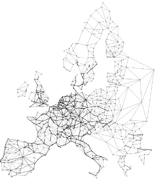
Figure 2. European11 quadrimodal graph
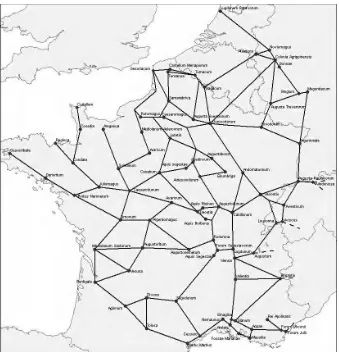
Figure 3.
Walte
r Christalle
Road network Highways and express routes
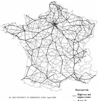
Route 70 Route 60 and 50 Ch. DECOUPIGNY, K. SERRHINI, CESA April 2000
Figure 4. Multimodal graph of France12
The search for the planarity of graphs led to famous publications and numerous algorithms. Among the best known results let us quote two traditional properties:
– Euler’s formula:
- let G be a connected planar simple graph with e edges and v vertices, - let r be the number of regions (or areas) in a planar representation of G. Then r = e – v + 2
– Kuratowski’s theorem: a graph is not planar if and only if it contains a homeomorphic subgraph with K3,3 or K5 (see Figure 5).
U1
U6
U2
U5 U4
U3 V1
V2
V4 V5
V3
Figure 5. K3,3 graph and K5 graph [ROS 98, p. 479 and 419]
We add two definitions to these traditional ones in order to specify graph plottings with more than two dimensions.
Graph with geographical reference
A graph with geographical reference “GGR” is either a plane graph or a graph plotted on a simple surface, for which it is possible to perform a bijection between the nodes of the plotting and those of its projection onto a plane. In other words, no node or face of a GGR must have a double point as a projection.
belongs to a surface defined in a three-dimensional space which is qualified by the use of the 2.5 dimension in landscape analysis13.
Graph with spatial reference
We will also call a graph with space reference, or GSR, a graph plotted on a convex surface or in a three-dimensional space or more, such as, for example, the solids of Plato but also the GSR like those used by Kamal Serrhini to define co-visibilities [SER 00]14. In this case, when the graph is projected onto a plane there does not have to be a bijection between the drawing of the graph in the space and its plane projection because certain points, nodes or areas can be doubled15. Let us note that the use sometimes qualifies the graphs drew on a “planar” sphere by extension, since in this case the plane is considered as a sphere with infinite radius.
Figure 6. Digital terrain model of the Mount Blanc [BRU 87]
13 This qualification, i.e. dimension 2.5, is usual and established by the use in co-visibility. It should be specified that it is used to differentiate this type of GGR grid from the GSR defined hereafter, which, in turn, is not limited by the constraint of bijection. This qualification of dimension 2.5 has nothing to do with a non-integer dimension of the fractal type.
14 See below Part 2, Chapter 10.
Dual graph
There exist many definitions of duality16. We will retain the one used by the majority of authors. The duality of a graph consists of associating each area of a graph called primal to a node of the dual graph. Berge provides the following definition for it [BER 87]: “let us consider a planar graph G, which is connected and without isolated nodes. We make it correspond to a planar graph G* in the following manner: inside every face s of G we place a node x * of G *; we make every edge e of G we correspond to an edge e* of G*, which connects the z nodes x* and y* corresponding to the faces s and t that are on both sides of edge e. The graph G* thus defined is planar connected and does not have an isolated node: it is called the dual graph of G” (see Figure 7).
Figure 7. Primal graph and its dual [BER 70]
This definition is insufficient and, for example, Aldous and Wilson specify [ALD 00]: “let G be a connected graph. Then a dual is constructed from a plane drawing (italics added) of G, as follows…”. The definition is more exact, as they demonstrate, by defining the dual of a convex three-dimensional polyhedron, as we examine in Part 3.
Similarly, in certain, even very simple, cases the dual is not of the same type as the primal in the sense that a primal 1-graph can have a p-graph as a dual, as we will see. This may present a problem in terms of graph description, since the adjacency matrix of the dual then has to be an extremely hollow p-dimensional matrix…
The concept of a dual graph is very rich, but insufficiently used. Indeed, it makes it possible to make areas correspond to networks and vice versa, which is one of the fundamental problems of synthesized images and of specialized network representations among others. Thanks to the duality and to what stems from it, it is possible to bypass some of the limitations facing modeling.
A particular type of graphs: the tree and tree structure
A tree is a connected undirected graph without a simple circuit. An undirected graph is a tree, if and only if each pair of nodes is connected by a simple and single circuit.
Tree and tree structure: we can call a particular node of the tree the root and then attribute a direction to each node in such a way that there is a only path from the root to each node. We then obtain a directed graph which is referred to as a tree structure (see Figure 8).
If v is a node other that the root, the father of v is the single node u, such that there is a directed arc from u to v. If u is the father of v, v is called the child of u. Nodes with the same father are called siblings. The ancestors of a node other than the root are nodes of the path leading from the root to this node. The descendants of a node v are the nodes that have v as ancestor. The node of a tree that does not have offspring is called a leaf. Nodes that have offspring are called internal nodes. A subtree is the subgraph comprised of a node of the tree, its descendants and all the arcs leading to its descendants.
A tree structure is described as m-ary if each internal node does not have more than m offspring. The tree is called a complete m-ary tree if each internal node has exactly m descendants. An m-ary tree with m = 2 is called a binary tree.
A tree structure will be quasi-strongly connected if there is a node u, from which we can reach all the others via a path. The node u is known as the root of the tree: it is the common ancestor of all the nodes.
An example of a tree structure in networks is a monopolar access map, such as those plotted by Laurent Chapelon17, or Legrand’s star map presented below (see Figure 9)
Some additional theorems deserve being mentioned: – a tree with n nodes contains n-1 arcs;
– a complete m-ary tree with i internal nodes contains n = mi + 1 nodes; – a complete m-ary tree with:
- n nodes contains i = (n-1)/m internal nodes and l = [(m-1) n + 1]/m leaves, - i internal nodes contains l = (m-1) i + 1 leaves,
- l leaves contains n = (ml-1)/(m-1) nodes and i = (l-1)/(m-1) internal nodes.
Figure 9. Merchandise traffic by rail in France. Annual throughput by line section (in effective thousands of tons) in 1854. Extract from Renouard, Les transports
des merchandises depuis 1850, Armand Colin
Spanning tree
Let G be a simple graph. A covering tree of G is a subgraph of G, which is a tree containing each node of G. Finally, a simple graph is connected if and only if it has a spanning tree.
The great algorithmic simplicity of graph theory is the heritage of operational research. Numerous problems that arise in the network simulation have been solved by operational research [FIN 08, KAU 64], which developed many algorithms first for a manual and then for a computerized resolution.
Among many publications that have made it possible to obtain effective algorithms it is necessary to cite Ford and Fulkerson for the flow algorithm in graphs, Dantzig and then Ford for the first shortest paths algorithms, etc. These works paved the way for many later achievements that have been encouraged and reinforced by developments in data processing, which provided the necessary means of computation.
Graph description methods for computer by list or by adjacency or incidence matrix, and all the methods derived from those easily lend themselves to the computerized processing and thus to the resolution of problems involving large graphs.
The use of these methods of computerized graph description has been made even simpler since the 1990s in the domain of transport networks by the development of data capture methods and the development of adjacency list-type files through the digitalization of maps or direct on-screen capture and modification (Chapelon, Les logiciels MAP et NOD [MAP and NOD Software]; see Chapelon, L’Hostis). The rapid development and generalization of GIS (geographical information systems) or of SRIS (spatial reference information systems) reinforce and accelerate this evolution.
power of n, which is the size of the problem, when n→∞…” [MIN 86]. For example, the time needed for the research of the minimal paths between any pair of nodes in a graph by Floyd’s algorithm [COR 94, p. 550] grows according to the cube of the number of nodes. In this algorithm that has an exceptionally beautiful symmetry of expression, there are three overlapping loops and when the number of nodes doubles, the computing time increases eightfold. It is an algorithm of complexity O(n3), that is, a polynomial complexity [ROS 98, p. 97 et seq.].
On the other hand, although computers have progressed considerably in their capacities to rapidly produce high definition images, this problem has practically not been tackled by graph theory whose development logic remains largely marked by its history and dependant on the research logic of mathematicians and operational researchers who are practically unaware of this aspect.
However, the fastest method to apprehend networks and results expressed as networks is the synthesized image, i.e. an effective and precise graphic representation, which is reproducible and verifiable to the same extent as the optimization calculations of operational and therefore algorithmic research. In spatial analysis and urban development planning the synthesized images must become a measurement and diagnostic instrument, as in many other disciplines: medicine, physics, biology, etc.
The representation of networks by graphs
Network modeling by graphs constitutes a relatively recent application for an old requirement. Although the network in its current meaning is a relatively modern concept, the need to represent a set of roads and terrestrial or maritime routes, on the other hand, is very old and has become accentuated with time. Indeed, this need develops along with the progressive interpenetration of societies witnessing the development of their exchanges. Little by little, tradesmen, sailors, soldiers will feel a greater need for not being dependant on local guides, for no longer being limited by local knowledge and for being able to consider all of the characteristics of various displacements: difficulty, length, duration, risk, locally available resources, etc. That explains the development of cartographic representation methods rather than networks and spaces.
From functional representation to resemblance
reached us thanks to a medieval copyist) which represents a map of ancient routes from city to city with the indication of distances.
Figure 11. Layout of the network of the Peutinger Table against the background of a modern map
Indeed, we note that it strictly corresponds to the definition of a graph plotting provided by Berge: “it is only necessary to know how the nodes are connected”. The Peutinger Table only slightly resembles a map and its representation against the background of a map18, whose form corresponds to that of the territory as above, makes it possible to see the differences (see Figure 11). These two representations are isomorphic but neither one nor the other has the properties of reproducibility and comparability. We could think that the second is very close to having these properties, but it is simply the force of habit that makes us forget all the implicit notions that it uses, such as, for example, the localization of nodes identical to the localization of cities, which results from these “stages mentioned in the table…”. The proof of this assertion is very simple and to observe it would suffice to ask a student, who is unaware of all the graphic semiology, to draw this map.
A millennium later, starting from the 13th and 14th centuries, the first portulans19 established by the Genoese and Venetian and then by Arabic and Portuguese navigators, illustrated the famous pilot’s logbooks thus showing that the description of the possible route must be accompanied by a representation, a graphic drawing and that the text is not enough20.
This need for cartographic representations supplementing the “nautical instructions” kept developing with the great discoveries and would constitute an extraordinarily important tool at sea and then on solid ground. Was it not Napoleon who considered the map as a weapon?
Increasingly scientific mapping
A considerable progress in precision, in semiological and mathematical rigor in the increasingly objectified maps has been carried out, among others, under the influence of the geometricians, of whom the Cassinis21 were undoubtedly the most famous. The triangulation of a space thus corresponds to defining a saturated planar graph in this space.
18 This map has been plotted in 2001 by Olivier Marlet, a student of “Urban Sciences” DEA archeology option at Tours.
19 From the Italian portulano: pilot.
20 Indeed, if machine descriptions of graphs as adjacency matrix, for example, enable many calculations including those of certain “morphological” indicators, they do not make it possible for the human mind to visualize the specific network, which is described without additional data…
However, between the sea or terrestrial maps and the Peutinger Table there is a fundamental difference: maps have the aim of representing the territory (i.e., amongst other things, a surface) in the most precise possible way: the relief of the depths or altitudes, its form (plateaus, mountains, peaks, reefs, cliffs, crossing points, major and minor rivers, currents, etc.), whereas the Peutinger Table is only a functional representation and does not resemble road networks.
Even if the map resulting from the Cassinis features the road communication networks, its aim is different: one of its constraints is that of “resemblance” to the territory because it must describe it and not be limited to networks, to “paths and circuits” in the sense of graphs, but also make it possible for someone to orientate himself in this terrestrial or maritime space. It is a tool to define the position in space in the most precise possible way.
This constraint of resemblance between the terrestrial surface and a plane representation was the object of many mathematical works and the development of the most traditional projection methods as those of Mercator22 and Lambert.
This objective of resemblance that the maps are given with the aim of representing the space or the territory implies the existence of homeomorphism between the space represented and the representation of space23. This property of homeomorphism doubles on maps due to a resemblance resulting from graphic semiology codes: the forests are in green, the rivers, the lakes and the seas in blue, etc. Even on a small scale Michelin map, the winding roads are represented with many turns indicating their sinuosity, etc. We are relatively far from Peutinger’s functional representation, even though it features some zigzags, stylized mountains and urban monuments.
Already overloaded with stylized decorations, fantastic characters and animals to fill in the blanks and to compensate for the unknowns, the map is overloaded with descriptive details of the territory by means of graphic semiology: the map has to account for the territory and it must make it possible to apprehend it as a whole, its evolution and its significant details. We refer to this as the constraints of resemblance.
22 Mercator Gerhard 1521-1594 Tabulae geographicae ad mentem Cl. Ptolemaei (1578) - Mercator readopts the projection invented in the 1st century by Martin de Tyr. This projection on a cylinder tangent to the equator is improved by Lambert who uses a cone tangent to a central meridian line.
Networks, roadmaps and graphs: the constraints of resemblance
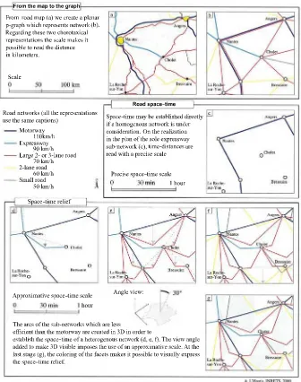
The maps representing networks must give the same impression of immediate resemblance, thus enabling an instantaneous comprehension. Undoubtedly, it is for this reason that the layout of a road on the Michelin map evokes the real layout of the road: straight where it is actually straight and curving when the layout is winding. Having said that, there is no strict relation between the two layouts because the width of the route is not connected with that of the representation but only bears a similarity: bolder lines for highways, thinner for minor roads, etc. Also, the smaller the scale of the map, the larger the disproportion becomes, which necessarily requires a simplified layout (Figure 12).
Figure 12. Evolution of a coastal layout through the reduction of the scale of representation
Networks, tree structures, flow charts: the constraints of hierarchy
The described networks can be of particular types, such as flow charts retracing a hierarchical system in a structure. The usage dictated by habit encourages a representation of this type of dissymmetrical network in a pyramidal form, with the most important element in the hierarchy sitting atop and the subordinate levels following each other in order of decreasing importance.
hereafter be referred to as data flow charts [FAU 75], which are graphic translations of a program or of a part of a program.
Many domains are still insufficiently explored
Graph theory primarily developed in two research directions: mathematical research and operational research, according to the specific dynamics of these two fields. The concerns and the questions posed by mathematicians are very specific, but often have very little to do with those of the developers of transport networks, space analysts and urban planners.
The concerns of the operational researchers are much closer to them. Some are obviously common, but urban planners, as those for whom their work is meant, i.e. contractors and the public, have a visualization requirement that cannot be circumvented and a need for illustration that, except in rare cases, is not present for operational researchers.
Urban planners need representations that are repetitive and verifiable, as well as comprehensible for all the public, in particular, within the framework of public interest investigations. Moreover, we have seen that graph theory is absolutely not preoccupied with the representation in the sense of graphic plotting of a graph. In a certain manner Berge eliminates the problem by writing: “it is only necessary to know how the nodes are connected. The localization of the nodes in the figure, the representation or plotting of the graph do not count” [BER 70, BER 87].
It is neither considered nor even mentioned that the representation can be “plotted” on a plane or in a three-dimensional space or be the projection of one onto the other [CAU 76, CAU 86], except in the case of a planar graph and that of the construction of a dual graph, which can be plotted on a plane, a sphere or a torus [HEA 76, HEA 86, LHU 76, LHU 86, POI 76, POI 86]. The concerns of the founding fathers of graph theory have been simultaneously developed and reduced. The drawing of graphs and their constraints, network image or images
This absence of rules of graph drawing is a considerable difficulty for the representation of modeled networks, whereas for network cartography there is a graphic semiology.
We propose as a working hypothesis that this definition will enable us to integrate various geometrical results into graph theory, in particular, certain basic elements of fractals that will make it possible to provide the rules for the extension or reduction of graphs, to ground in theory the already operational concept of zoom by using the property of self similarity or strict or probabilistic internal homothety and to provide global morphological indicators of networks, such as the fractal dimension [GEN 00].
The problem of graph extension and reduction and the scales of representation under constraints are very important problems in network modeling. We have mentioned the complexity of the algorithms for the resolution of traditional problems, such as that of the search for the shortest paths in a graph, and also mentioned that it was of the O(n3) level. It is then easily conceived that two problems present themselves acutely: that of the reduction of large graphs and that of the rule to be used for the process not to be left completely to the free interpretation of the modeler, but to be, as we have already stated, reproducible and verifiable; basically, to be more objective, more scientific.
This problem of reduction of graphs and of the size of graphs to be processed, even though it evolves rapidly with the performance of machines, ipso facto poses the problem of the levels of calculation or the scales in spatial analysis. The problem of the existence of various network apprehension and modeling scales immediately leads to the question of the existence of internal homothety between the various levels considered. Can they be treated in the same manner and up to which point, which limit?
We pose the working hypothesis that at a certain level the logic and the hypotheses change. For example, the reflection on the saturation of a transport system can be solved by calculating the capacity of one or several cross-sections of the network by using the Ford-Fulkerson theorem. However, this is done at the cost of very strong assumptions and, in particular, those according to which the node is strictly neutral, which is the general assumption in graph theory that only deals with the relationships between nodes and not with them as such. Consequently, the saturation of an arc is related to its capacity. This is obviously at the very least an abusive assumption and completely opposed to the reality of the flux of flows. Any car driver knows from experience that the saturation of an axis almost always results from the saturation of a crossroads, i.e. of a node, except for cases that constitute an accident, like the reduction of the number of lanes, and even in this last case, normally, the capacity of an arc should equal that of its narrowest portion.
example, the highway half-interchange24 obviously exists and yet it is impossible to represent it by a node under the current state of the theory.
Therefore, it is necessary to improve network modeling, to call into question this assumption of the neutrality of nodes and to consider their structures, the possibility of describing them while respecting the axioms and fundamental properties of graph theory.
We put forward another working hypothesis: the development of drawing rules, of representation as well as a reflection on the duality must make it possible to pass from the traditional graph to percolation and the use of MSA (multi-agent systems) in a cellular network, with all the modifications of hypotheses with respect to application that this enables and implies. Indeed, to describe and to simulate, even to optimize, as a whole,, a transport system is a type of problem that implies certain assumptions that we will clarify; on the other hand, describing the individual behavior of an agent in a network is another problem and does not necessarily require the same assumptions, since sometimes it renders them particularly illusory. Similarly, even thought graph theory indeed makes it possible to represent a network with facility and flexibility and with a certain degree of generality in order to solve some of the problems mentioned above, it enables very little with respect to the graph area which is enclosed between its various arcs.
That is obvious because graph theory is only preoccupied with the relations between nodes. However, the property of duality makes it possible to take this space into account. Nonetheless, this property is closely related to the planar representation of the graph and therefore requires a certain number of additional hypotheses and the contribution of additional precise details in order to answer the questions posed above. This problem will be tackled later in the book.
Lastly, one of the problems that dynamic network modeling comes across is the development of networks, the extension of the graph and of its grid, either simultaneously or subsequently.
We will see that the possibility of describing simple fractals as graphs makes it possible to find a solution for these problems.
If we wish, as is the case, to be able to achieve comparable and repetitive drawing and, thus, the layout of maps in Waldo Tobler’s sense, we will note that additional assumptions are necessary to specify the type of possible layout.
Similarly, we observe that with some additional assumptions and constraints we are able to drow graphs that have all the properties of fractals.
An explicit assumption must be stressed due to its consequences on later applications: in graph theory we adopt the hypothesis of perfect rationality and total knowledge of the network. Indeed, let there be a graph corresponding to the definition above, where all its elements are known to us via a complete and finite list of nodes and that of the relations between nodes, which is described by the list or the adjacency matrix. Such a definition is absolutely necessary to be able to deal with the basic problems of graph theory and, in particular, the problems of optimization of paths and maximum flow. The demonstration is obvious: if a single arc was missing, it would be impossible to obtain the matrix of the minimal path, since at least one of them might not exist if an arc was added. A fortiori if a node is missing.
This significant hypothesis is no longer necessary for the simulation of agents in a “cellular graph”: in order to find a path, the local knowledge such as, for example, the number of arcs starting at the node or the next node and their orientations with respect to a reference direction may suffice. The set of necessary assumptions will thus have to be specified for each application and each representation of the graphs. The plan
The plan of the book follows the development of the questions that we have touched upon above and comprises three parts: the first is entitled Graph theory and network modeling; the second, Graph theory and network representation and the third, Towards a multilevel graph theory.
Bibliography
[ALD 00] ALDOUS J.M., WILSON R.J., Graphs and Applications, an Introductory Approach, Springer-Verlag, London, Berlin, Heidelberg, 2000.
[BEA 92] BEAUQUIER D., BERSTEL J., CHRETIENNE P., Eléments d’algorithmique, Masson, 1992.
[BER 70] BERGE C., Graphes, Dunod, Paris, 1970. [BER 87] BERGE C., Hyper graphes, Bordas, Paris, 1987.
[BRU 87] BRUNET R., La carte mode d’emploi, Fayard/Reclus, Paris, 1987.
[CAU 86] CAUCHY A.L., “Recherches sur les polyèdres”, Premier mémoire J. Ecole Polytechnique 9 (Cah.16) (1813), p. 68-86., in N.L. Biggs, E.K. Lloyd and R.J. Wilson, Graph theory 1736-1936, Oxford University Press, 1976, 1986.
[CHO 64] CHOW Y., CASSIGNOL E., Théorie et application des graphes de transfert, Dunod, 1964.
[CHR 33] CHRISTALLER W., Die zentralen Orte in Sûddeutschland, G. Fischer, Paris, 1933.
[COR 94] CORMEN T., LEISERSON C., RIVEST R., Introduction à l’algorithmique, Dunod, Paris, 1994.
[EUL 1736] EULER L., “Solutio problemats ad geometriam situs pertitnentis”, Commemtarii Academia Scientiarum Imperialis Petropolitanae, 8, p 128-140, Opera Omnia, vol. 7, p. 1-10, 1736.
[EUL 1758a] EULER L., “Demonstreatio nonnullarum insignium proprietatum quibus solidra hedris planis inclusa sunt praedita”, Novi Comm. Acad. Sci. Imp. Petropl. 4 (1752-1753, published in 1758), 140-160, Opera Omnia (1), vol. 26, 94-108, 1758.
[EUL 1758b] EULER L., Elementa doctrina solidorum. Novi Comm Acad. SCI. Imp. Petropol. 4 (1752-1753, published in 1758), 109-140, Opera Omnia (1) vol. 26, 72-93, 1758.
[FAU 75] FAURE R., Eléments de recherche opérationnelle, Collection “Programmation”, Gauthier-Villars, Paris, 1975.
[FIN 08] FINKE G., Operations Research and Networks, ISTE, London, John Wiley &Sons, New York, 2008.
[FOR 68] FORD L.R.Jr., FULKERSON D.R., Les flots dans les graphes trad, J.C. Arinal (dir.) Gauthier-Villars, Paris, 1968, Flows in networks, RAND Corporation, 1962, Princeton University Press.
[GEN 00] GENRE GRANDPIERRE C., Forme et fonctionnement des réseaux de transport : approche fractale et réflexions sur l’aménagement des villes, PhD Thesis, Besançon, 2000.
[HEA 86] HEADWOOD P.J., “Map Colour Theorem”, Quaterly Journal of Pure and Applied Mathematics 24 (1890), 332-338, Graph theory 1736-1936 Biggs N.L., Lloyd E.K., Wilson R.J., Oxford University Press, 1976, 1986.
[KAU 64] KAUFMANN A., Méthode et modèles de la recherche opérationnelle, Vol. 1 and 2, Dunod, Paris, 1964.
[LHU 86] LHUILLIER S.6A.6J., “Mémoire sur la Polyédrométrie”, Annales de Mathématiques 3 (1812-3), p. 169-189, in Biggs N.L., Lloyd E.K., Wilson R.J., Graph theory 1736-1936 Oxford University Press, 1976, 1986.
[PUM 97] PUMAIN D., SAINT JULIEN T., Analyse spatiale 1 Localisations dans l’espace, Armand Colin, 1997.
[ROS 91] ROSEN K.H., Mathématiques discrètes, Chénelière/MCGraw-Hill, 1991.
[SER 00] SERRHINI K., Evaluation spatiale de la covisibilité d’un aménagement, sémiologie graphique expérimentale et modélisation quantitative, PhD Thesis, Tours, 2000.
Created by M. Appert, L. Chapelon, 2001, UMR 6012-ESPACE, Montpellier NOD/MAP software: L. Chapelon, L’Hostis, Ph. Mathis, CESA, 1993/2002
Created by M. Appert, L. Chapelon, 2001, UMR 6012-ESPACE, Montpellier NOD/MAP software: L. Chapelon, L’Hostis, Ph. Mathis, CESA, 1993/2002
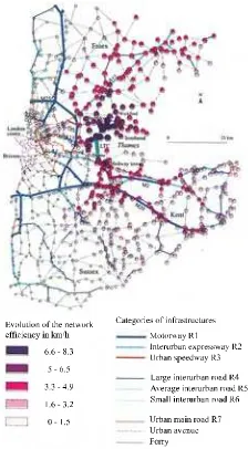
Figure 1.3. Graph of the road network in the
East Thames corridor
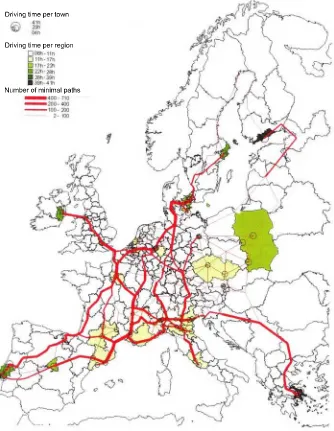
Figure 1.4. Sum of minimal driving times
Figure 1.5. Performance of the road network between 1 and 2 pm (off-peak)
Figure 1.6. Performance of the road network
between 5 and 6 pm (rush hour)
Created by M. Appert, L. Chapelon, 2001, UMR 6012-ESPACE, Montpellier NOD/MAP software: L. Chapelon, L’Hostis, Ph. Mathis, CESA, 1993/2002
Figure 1.7. Simulation of the performance results obtained
the DTM graph of Tanet
Figure 2.2. Realization of the graph of the path from DTM
Figure 2.4. Geomorphology of the theoretical DTM graph
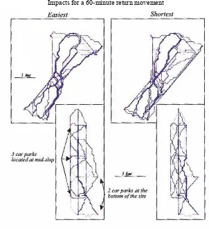
Impacts for a 60-minute single movement Impacts for a 60-minute return movement
Figure 2.5. Simulation of the movements on
the Tanet and theoretical space
Figure 2.6. Impacts of the movements on the
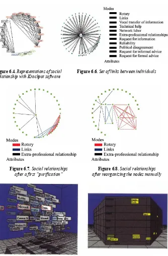
relationship with Krackpot software
Figure 6.7. Social relationships
after a first “purification”
Figure 6.8. Social relationships
after reorganizing the nodes manually
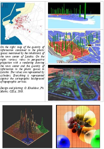
On the right: map of the quantity of information contained in the phatic spaces mentioned by the inhabitants of the town center of Latakia. On the right: various views in perspective projection with a rendering showing the town center and the quantity of information in the phatic spaces in Latakia. The values are represented by cylinders. Everything is represented against the cartographic background of topographic services.
Design and plotting: O. Khaddour, Ph. Mathis. CESA, 2003.
Figure 7.1. Various representations of the attractiveness of phatic
Ph. Mathis, K. Serrhini in collaboration with M. Mayaud (cartographer), CESA, January 2001
Figure 10.5. Covisibility from the green mesh of the A28 section
Figure 10.6. Space seen along the A28 section. Generalized visibility from the A28 section reported (in %) on the smoothed square (32 x 32) meshes of space
(section of the A28 at Chanceaux-sur-Choisille, Indre-et-Loire, 37)
Figure 10.7. Determination of the
topographic transversal (view: Plan (XY))
Figure 10.8. Anthropic generalized visibility.
the distance from the installation (A28 section at Chanceaux-sur-Choisille, Indre-et-Loire, 37)
Figure 10.10. Directed, dynamic and static
generalized visibility along the A28 section deferred (in % or in time) on the square
space meshes
Figure 10.11.
Primal graph, dual graph and
covisibility. Covisibility starting from the green mesh of the A28 section according to
two cities of equal population (potential market)
Figures 11.11 and 11.12. For each year: on the left, production surfaces for each product
(in red for product 1, in green for product 2 and in blue for product 3); on the right, market place where production is transported (all the domains that sell
paths by a blue line and the position of tourists on the beach by a blue dot; the sea at low tide is in light blue, and the colors on the dune refer to the coefficient of practicability
ranging from easy in white to impossible (barbed wire) in red
Figure 13.3. Crossing the dune area according to two different
to the digital model of the hill area, for a difficulty slope of 0%
Figure 13.5. Simulations of the percolative diffusions of tourists according
to the digital model of the hill area, for a difficulty slope of 14%
Figure 13.6. Simulations of the percolative diffusions of tourists according
PART 1
Chapter 1
The Space-time Variability of Road Base
Accessibility: Application to London
This chapter presents an attempt to integrate traffic conditions into an accessibility calculation model associated with road networks at the regional scale. For identical networks, congestion, which is closely linked to the use of infrastructure, is responsible for variations of traffic speeds. In order to optimize accessibility calculations it is of primary importance to obtain the “real” speed section by section by taking into account the level of traffic. To that end we endeavored to systemize the empirical approach initiated by the Transport Research Board and developed in its Highway Capacity Manual [TRB 98]. This approach, which is associated with a specific road network modeling method in the form of valuated graphs, can indeed account for space and time variability of motor vehicle traffic speed on roads.
1.1. Bases and principles of modeling
1.1.1. Modeling of the regional road network
Graph theory is one of the most effective means to model transport networks. The vertices of a graph are associated with network nodes and the arcs are associated with links. Along with the principle of mechanical graph description, this type of modeling makes it possible to benefit directly from the calculating power offered by computers.
1.1.1.1. From network to graph
A priori no constraints restrict the choice of the graph vertices. The size of nodes in terms of population, of economic or administrative functions, for example, may be given prevalence. However, several factors must be taken into account in order to improve the precision of the results.
First of all, the strategic role that certain nodes may play in the organization and operation of the road network (crossroads, interchanges) makes it necessary to compute them. Then, when the design features of the infrastructure or their environment (urban/rural) change, it is advisable to create a new arc. The vertices are placed consequently. Lastly, the graph can also adapt itself to the available structure of traffic measurement. The limits separating two measurements series are therefore likely to be regarded as vertices of the graph.
Optimally, an arc corresponds to a section of the road presenting relatively homogenous design features and intensity of use over its entire length.
The arcs of the graph must render with precision the design features of the road infrastructure, insofar as they directly influence the traffic speed. That relates simultaneously to the structure and the quality of the roads. Among the elements that may be noted let us cite the number, width, pattern, slope, sinuosity of lanes, existence of a central reservation on dual carriageways, width of lateral clearances, etc.
![Figure 6. Digital terrain model of the Mount Blanc [BRU 87]](https://thumb-ap.123doks.com/thumbv2/123dok/3934450.1877870/29.595.148.462.350.551/figure-digital-terrain-model-mount-blanc-bru.webp)