Digital Signal Processing
Digital Signal Processing
Second Edition
by
Steven W. Smith
Important Legal Information: Warning and Disclaimer
This book presents the fundamentals of Digital Signal Processing using examples from common science and engineering problems. While the author believes that the concepts and data contained in this book are accurate and correct, they should not be used in any application without proper verification by the person making the application. Extensive and detailed testing is essential where incorrect functioning could result in personal injury or damage to property. The material in this book is intended solely as a teaching aid, and is not represented to be an appropriate or safe solution to any particular problem. For this reason, the author, publisher, and distributors make no warranties, express or implied, that the concepts, examples, data, algorithms, techniques, or programs contained in this book are free from error, conform to any industry standard, or are suitable for any application. The author, publisher, and distributors disclaim all liability and responsibility to any person or entity with respect to any loss or damage caused, or alleged to be caused, directly or indirectly, by the information contained in this book. If you do not wish to be bound by the above, you may return this book to the publisher for a full refund.
Digital Signal Processing
Second Edition
by
Steven W. Smith
copyright © 1997-1999 by California Technical Publishing
All rights reserved. No portion of this book may be reproduced or transmitted in any form or by any means, electronic or mechanical, without written permission of the publisher.
ISBN 0-9660176-7-6 hardcover ISBN 0-9660176-4-1 paperback ISBN 0-9660176-6-8 electronic LCCN 97-80293
California Technical Publishing P.O. Box 502407
San Diego, CA 92150-2407
To contact the author or publisher through the internet: website: DSPguide.com
e-mail: [email protected]
Printed in the United States of America First Edition, 1997
v FOUNDATIONS
Chapter 1. The Breadth and Depth of DSP . . . 1
Chapter 2. Statistics, Probability and Noise . . . 11
Chapter 3. ADC and DAC . . . 35
Chapter 4. DSP Software . . . 67
FUNDAMENTALS Chapter 5. Linear Systems . . . 87
Chapter 6. Convolution . . . 107
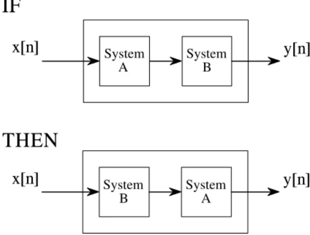
Chapter 7. Properties of Convolution . . . 123
Chapter 8. The Discrete Fourier Transform . . . 141
Chapter 9. Applications of the DFT . . . 169
Chapter 10. Fourier Transform Properties . . . 185
Chapter 11. Fourier Transform Pairs . . . 209
Chapter 12. The Fast Fourier Transform . . . 225
Chapter 13. Continuous Signal Processing . . . 243
DIGITAL FILTERS Chapter 14. Introduction to Digital Filters . . . 261
Chapter 15. Moving Average Filters . . . 277
Chapter 16. Windowed-Sinc Filters . . . 285
Chapter 17. Custom Filters . . . 297
Chapter 18. FFT Convolution . . . 311
Chapter 19. Recursive Filters . . . 319
Chapter 20. Chebyshev Filters . . . 333
Chapter 21. Filter Comparison . . . 343
APPLICATIONS Chapter 22. Audio Processing . . . 351
Chapter 23. Image Formation and Display . . . 373
Chapter 24. Linear Image Processing . . . 397
Chapter 25. Special Imaging Techniques . . . 423
Chapter 26. Neural Networks (and more!) . . . 451
Chapter 27. Data Compression . . . 481
Chapter 28. Digital Signal Processors . . . 503
Chapter 29. Getting Started with DSPs . . . 535
COMPLEX TECHNIQUES Chapter 30. Complex Numbers . . . 551
Chapter 31. The Complex Fourier Transform . . . 567
Chapter 32. The Laplace Transform . . . 581
Chapter 33. The z-Transform . . . 605
Glossary . . . 631
vi
FOUNDATIONS
Chapter 1. The Breadth and Depth of DSP . . . 1 The Roots of DSP 1
Telecommunications 4 Audio Processing 5 Echo Location 7 Imaging Processing 9
Chapter 2. Statistics, Probability and Noise . . . 11 Signal and Graph Terminology 11
Mean and Standard Deviation 13 Signal vs. Underlying Process 17 The Histogram, Pmf and Pdf 19 The Normal Distribution 26 Digital Noise Generation 29 Precision and Accuracy 32
Chapter 3. ADC and DAC . . . 35 Quantization 35
The Sampling Theorem 39 Digital-to-Analog Conversion 44 Analog Filters for Data Conversion 48 Selecting the Antialias Filter 55 Multirate Data Conversion 58 Single Bit Data Conversion 60
Chapter 4. DSP Software . . . 67 Computer Numbers 67
Fixed Point (Integers) 68
Floating Point (Real Numbers) 70 Number Precision 72
Execution Speed: Program Language 76 Execution Speed: Hardware 80
vii
Chapter 5. Linear Systems. . . 87 Signals and Systems 87
Requirements for Linearity 89
Static Linearity and Sinusoidal Fidelity 92 Examples of Linear and Nonlinear Systems 94 Special Properties of Linearity 96
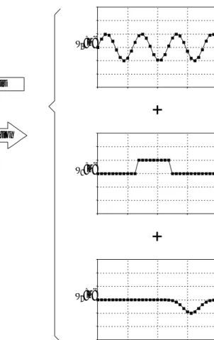
Superposition: the Foundation of DSP 98 Common Decompositions 100
Alternatives to Linearity 104
Chapter 6. Convolution . . . 107 The Delta Function and Impulse Response 107
Convolution 108
The Input Side Algorithm 112 The Output Side Algorithm 116 The Sum of Weighted Inputs 122
Chapter 7. Properties of Convolution . . . 123 Common Impulse Responses 123
Mathematical Properties 132 Correlation 136
Speed 140
Chapter 8. The Discrete Fourier Transform . . . 141 The Family of Fourier Transforms 141
Notation and Format of the real DFT 146
The Frequency Domain's Independent Variable 148 DFT Basis Functions 150
Synthesis, Calculating the Inverse DFT 152 Analysis, Calculating the DFT 156
Duality 161 Polar Notation 161 Polar Nuisances 164
Chapter 9. Applications of the DFT . . . 169 Spectral Analysis of Signals 169
Frequency Response of Systems 177 Convolution via the Frequency Domain 180
Chapter 10. Fourier Transform Properties . . . 185 Linearity of the Fourier Transform 185
Characteristics of the Phase 188 Periodic Nature of the DFT 194
viii
The Discrete Time Fourier Transform 206 Parseval's Relation 208
Chapter 11. Fourier Transform Pairs . . . 209 Delta Function Pairs 209
The Sinc Function 212 Other Transform Pairs 215 Gibbs Effect 218
Harmonics 220 Chirp Signals 222
Chapter 12. The Fast Fourier Transform . . . 225 Real DFT Using the Complex DFT 225
How the FFT Works 228 FFT Programs 233
Speed and Precision Comparisons 237 Further Speed Increases 238
Chapter 13. Continuous Signal Processing . . . 243 The Delta Function 243
Convolution 246
The Fourier Transform 252 The Fourier Series 255
DIGITAL FILTERS
Chapter 14. Introduction to Digital Filters. . . 261 Filter Basics 261
How Information is Represented in Signals 265 Time Domain Parameters 266
Frequency Domain Parameters 268
High-Pass, Band-Pass and Band-Reject Filters 271 Filter Classification 274
Chapter 15. Moving Average Filters . . . 277 Implementation by Convolution 277
Noise Reduction vs. Step Response 278 Frequency Response 280
Relatives of the Moving Average Filter 280 Recursive Implementation 282
Chapter 16. Windowed-Sinc Filters . . . 285 Strategy of the Windowed-Sinc 285
Designing the Filter 288
ix
Arbitrary Frequency Response 297 Deconvolution 300
Optimal Filters 307
Chapter 18. FFT Convolution . . . 311 The Overlap-Add Method 311
FFT Convolution 312 Speed Improvements 316
Chapter 19. Recursive Filters . . . 319 The Recursive Method 319
Single Pole Recursive Filters 322 Narrow-band Filters 326
Phase Response 328 Using Integers 332
Chapter 20. Chebyshev Filters . . . 333 The Chebyshev and Butterworth Responses 333
Designing the Filter 334 Step Response Overshoot 338 Stability 339
Chapter 21. Filter Comparison . . . 343 Match #1: Analog vs. Digital Filters 343
Match #2: Windowed-Sinc vs. Chebyshev 346 Match #3: Moving Average vs. Single Pole 348
APPLICATIONS
Chapter 22. Audio Processing . . . 351 Human Hearing 351
Timbre 355
Sound Quality vs. Data Rate 358 High Fidelity Audio 359
Companding 362
Speech Synthesis and Recognition 364 Nonlinear Audio Processing 368
Chapter 23. Image Formation and Display. . . 373 Digital Image Structure 373
Cameras and Eyes 376 Television Video Signals 384
Other Image Acquisition and Display 386 Brightness and Contrast Adjustments 387 Grayscale Transforms 390
x
Convolution 397
3×3 Edge Modification 402 Convolution by Separability 404
Example of a Large PSF: Illumination Flattening 407 Fourier Image Analysis 410
FFT Convolution 416
A Closer Look at Image Convolution 418
Chapter 25. Special Imaging Techniques . . . 423 Spatial Resolution 423
Sample Spacing and Sampling Aperture 430 Signal-to-Noise Ratio 432
Morphological Image Processing 436 Computed Tomography 442
Chapter 26. Neural Networks (and more!) . . . 451 Target Detection 451
Neural Network Architecture 458 Why Does it Work? 463
Training the Neural Network 465 Evaluating the Results 473 Recursive Filter Design 476
Chapter 27. Data Compression . . . 481 Data Compression Strategies 481
Run-Length Encoding 483 Huffman Encoding 484 Delta Encoding 486 LZW Compression 488
JPEG (Transform Compression) 494 MPEG 501
Chapter 28. Digital Signal Processors . . . 503 How DSPs are different 503
Circular Buffering 506
Architecture of the Digital Signal Processor 509 Fixed versus Floating Point 514
C versus Assembly 520 How Fast are DSPs? 526
The Digital Signal Processor Market 531
Chapter 29. Getting Started with DSPs . . . 535 The ADSP-2106x family 535
The SHARC EZ-KIT Lite 537
xi
Advanced Software Tools 546
COMPLEX TECHNIQUES
Chapter 30. Complex Numbers . . . 551 The Complex Number System 551
Polar Notation 555
Using Complex Numbers by Substitution 557 Complex Representation of Sinusoids 559 Complex Representation of Systems 561 Electrical Circuit Analysis 563
Chapter 31. The Complex Fourier Transform . . . 567 The Real DFT 567
Mathematical Equivalence 569 The Complex DFT 570
The Family of Fourier Transforms 575
Why the Complex Fourier Transform is Used 577
Chapter 32. The Laplace Transform. . . 581 The Nature of the s-Domain 581
Strategy of the Laplace Transform 588 Analysis of Electric Circuits 592 The Importance of Poles and Zeros 597 Filter Design in the s-Domain 600
Chapter 33. The z-Transform . . . 605 The Nature of the z-Domain 605
Analysis of Recursive Systems 610 Cascade and Parallel Stages 616 Spectral Inversion 619
Gain Changes 621
Chebyshev-Butterworth Filter Design 623 The Best and Worst of DSP 630
xii
Goals and Strategies of this Book
The technical world is changing very rapidly. In only 15 years, the power of personal computers has increased by a factor of nearly one-thousand. By all accounts, it will increase by another factor of one-thousand in the next 15 years. This tremendous power has changed the way science and engineering is done, and there is no better example of this than Digital Signal Processing.
In the early 1980s, DSP was taught as a graduate level course in electrical engineering. A decade later, DSP had become a standard part of the undergraduate curriculum. Today, DSP is a basic skill needed by scientists and engineers in many fields. Unfortunately, DSP education has been slow to adapt to this change. Nearly all DSP textbooks are still written in the traditional electrical engineering style of detailed and rigorous mathematics. DSP is incredibly powerful, but if you can't understand it, you can't use it!
This book was written for scientists and engineers in a wide variety of fields: physics, bioengineering, geology, oceanography, mechanical and electrical engineering, to name just a few. The goal is to present practical techniques while avoiding the barriers of detailed mathematics and abstract theory. To achieve this goal, three strategies were employed in writing this book:
First, the techniques are explained, not simply proven to be true through mathematical derivations. While much of the mathematics is included, it is not used as the primary means of conveying the information. Nothing beats a few well written paragraphs supported by good illustrations.
xiii
C, Fortran, or a similar language. However, learning DSP has different requirements than using DSP. The student needs to concentrate on the algorithms and techniques, without being distracted by the quirks of a particular language. Power and flexibility aren't important; simplicity is critical. The programs in this book are written to teach DSP in the most straightforward way, with all other factors being treated as secondary. Good programming style is disregarded if it makes the program logic more clear. For instance:
‘ a simplified version of BASIC is used
‘ line numbers are included
‘ the only control structure used is the FOR-NEXT loop
‘ there are no I/O statements
This is the simplest programming style I could find. Some may think that this book would be better if the programs had been written in C. I couldn't disagree more.
The Intended Audience
This book is primarily intended for a one year course in practical DSP, with the students being drawn from a wide variety of science and engineering fields. The suggested prerequisites are:
‘ A course in practical electronics: (op amps, RC circuits, etc.)
‘ A course in computer programming (Fortran or similar)
‘ One year of calculus
This book was also written with the practicing professional in mind. Many everyday DSP applications are discussed: digital filters, neural networks, data compression, audio and image processing, etc. As much as possible, these chapters stand on their own, not requiring the reader to review the entire book to solve a specific problem.
Support by Analog Devices
The Second Edition of this book includes two new chapters on Digital Signal
Processors, microprocessors specifically designed to carry out DSP tasks. Much of
xiv
A special thanks to the many reviewers who provided comments and suggestions on this book. Their generous donation of time and skill has made this a better work: Magnus Aronsson (Department of Electrical Engineering, University of Utah); Bruce B. Azimi (U.S. Navy); Vernon L. Chi (Department of Computer Science, University of North Carolina); Manohar Das, Ph.D. (Department of Electrical and Systems Engineering, Oakland University); Carol A. Dean (Analog Devices, Inc.); Fred DePiero, Ph.D. (Department of Electrical Engineering, CalPoly State University); Jose Fridman, Ph.D. (Analog Devices, Inc.); Frederick K. Duennebier, Ph. D. (Department of Geology and Geophysics, University of Hawaii, Manoa); D. Lee Fugal (Space & Signals Technologies); Filson H. Glanz, Ph.D. (Department of Electrical and Computer Engineering, University of New Hampshire); Kenneth H. Jacker, (Department of Computer Science, Appalachian State University); Rajiv Kapadia, Ph.D. (Department of Electrical Engineering, Mankato State University); Dan King (Analog Devices, Inc.); Kevin Leary (Analog Devices, Inc.); A. Dale Magoun, Ph.D. (Department of Computer Science, Northeast Louisiana University); Ben Mbugua (Analog Devices, Inc.); Bernard J. Maxum, Ph.D. (Department of Electrical Engineering, Lamar University); Paul Morgan, Ph.D. (Department of Geology, Northern Arizona University); Dale H. Mugler, Ph.D. (Department of Mathematical Science, University of Akron); Christopher L. Mullen, Ph.D. (Department of Civil Engineering, University of Mississippi); Cynthia L. Nelson, Ph.D. (Sandia National Laboratories); Branislava Perunicic-Drazenovic, Ph.D. (Department of Electrical Engineering, Lamar University); John Schmeelk, Ph.D. (Department of Mathematical Science, Virginia Commonwealth University); Richard R. Schultz, Ph.D. (Department of Electrical Engineering, University of North Dakota); David Skolnick (Analog Devices, Inc.); Jay L. Smith, Ph.D. (Center for Aerospace Technology, Weber State University); Jeffrey Smith, Ph.D. (Department of Computer Science, University of Georgia); Oscar Yanez Suarez, Ph.D. (Department of Electrical Engineering, Metropolitan University, Iztapalapa campus, Mexico City); and other reviewers who wish to remain anonymous.
This book is now in the hands of the final reviewer, you. Please take the time to give me your comments and suggestions. This will allow future reprints and editions to serve your needs even better. All it takes is a two minute e-mail message to: [email protected]. Thanks; I hope you enjoy the book.
1
1
The Breadth and Depth of DSP
Digital Signal Processing is one of the most powerful technologies that will shape science and engineering in the twenty-first century. Revolutionary changes have already been made in a broad
range of fields: communications, medical imaging, radar & sonar, high fidelity music reproduction, and oil prospecting, to name just a few. Each of these areas has developed a deep
DSP technology, with its own algorithms, mathematics, and specialized techniques. This combination of breath and depth makes it impossible for any one individual to master all of the DSP technology that has been developed. DSP education involves two tasks: learning general concepts that apply to the field as a whole, and learning specialized techniques for your particular area of interest. This chapter starts our journey into the world of Digital Signal Processing by describing the dramatic effect that DSP has made in several diverse fields. The revolution has begun.
The Roots of DSP
Digital Signal Processing is distinguished from other areas in computer science by the unique type of data it uses: signals. In most cases, these signals originate as sensory data from the real world: seismic vibrations, visual images, sound waves, etc. DSP is the mathematics, the algorithms, and the techniques used to manipulate these signals after they have been converted into a digital form. This includes a wide variety of goals, such as: enhancement of visual images, recognition and generation of speech, compression of data for storage and transmission, etc. Suppose we attach an analog-to-digital converter to a computer and use it to acquire a chunk of real world data. DSP answers the question: What next?
DSP
Space
Medical
Commercial
Military
Scientific
Industrial
Telephone
-Earthquake recording & analysis -Data acquisition
-Spectral analysis -Simulation and modeling -Oil and mineral prospecting -Process monitoring & control -Nondestructive testing -CAD and design tools -Radar
-Sonar
-Ordnance guidance -Secure communication -Voice and data compression -Echo reduction
-Signal multiplexing -Filtering
-Image and sound compression for multimedia presentation -Movie special effects -Video conference calling -Diagnostic imaging (CT, MRI, ultrasound, and others) -Electrocardiogram analysis -Medical image storage/retrieval -Space photograph enhancement -Data compression
-Intelligent sensory analysis by remote space probes
FIGURE 1-1
DSP has revolutionized many areas in science and engineering. A few of these diverse applications are shown here.
data are irreplaceable; and medical imaging, where lives could be saved. The personal computer revolution of the 1980s and 1990s caused DSP to explode with new applications. Rather than being motivated by military and government needs, DSP was suddenly driven by the commercial marketplace. Anyone who thought they could make money in the rapidly expanding field was suddenly a DSP vender. DSP reached the public in such products as: mobile telephones, compact disc players, and electronic voice mail. Figure 1-1 illustrates a few of these varied applications.
This technological revolution occurred from the top-down. In the early 1980s, DSP was taught as a graduate level course in electrical engineering. A decade later, DSP had become a standard part of the undergraduate
Digital
Signal
Processing
Communication Theory
Analog
Electronics DigitalElectronics
Probability and Statistics
Decision Theory
Analog Signal Processing Numerical Analysis
FIGURE 1-2
Digital Signal Processing has fuzzy and overlapping borders with many other areas of science, engineering and mathematics.
in many fields. As an analogy, DSP can be compared to a previous technological revolution: electronics. While still the realm of electrical engineering, nearly every scientist and engineer has some background in basic circuit design. Without it, they would be lost in the technological world. DSP has the same future.
This recent history is more than a curiosity; it has a tremendous impact on your
ability to learn and use DSP. Suppose you encounter a DSP problem, and turn to textbooks or other publications to find a solution. What you will typically find is page after page of equations, obscure mathematical symbols, and unfamiliar terminology. It's a nightmare! Much of the DSP literature is baffling even to those experienced in the field. It's not that there is anything wrong with this material, it is just intended for a very specialized audience. State-of-the-art researchers need this kind of detailed mathematics to understand the theoretical implications of the work.
A basic premise of this book is that most practical DSP techniques can be learned and used without the traditional barriers of detailed mathematics and theory. The Scientist and Engineer’s Guide to Digital Signal Processing is written for those who want to use DSP as a tool, not a new career.
Telecommunications
Telecommunications is about transferring information from one location to another. This includes many forms of information: telephone conversations, television signals, computer files, and other types of data. To transfer the information, you need a channel between the two locations. This may be a wire pair, radio signal, optical fiber, etc. Telecommunications companies receive payment for transferring their customer's information, while they must pay to establish and maintain the channel. The financial bottom line is simple: the more information they can pass through a single channel, the more money they make. DSP has revolutionized the telecommunications industry in many areas: signaling tone generation and detection, frequency band shifting, filtering to remove power line hum, etc. Three specific examples from the telephone network will be discussed here: multiplexing, compression, and echo control.
Multiplexing
There are approximately one billion telephones in the world. At the press of a few buttons, switching networks allow any one of these to be connected to any other in only a few seconds. The immensity of this task is mind boggling! Until the 1960s, a connection between two telephones required passing the analog voice signals through mechanical switches and amplifiers. One connection required one pair of wires. In comparison, DSP converts audio signals into a stream of serial digital data. Since bits can be easily intertwined and later separated, many telephone conversations can be transmitted on a single channel. For example, a telephone standard known as the T-carrier system can simultaneously transmit 24 voice signals. Each voice signal is sampled 8000 times per second using an 8 bit companded (logarithmic compressed) analog-to-digital conversion. This results in each voice signal being represented as 64,000 bits/sec, and all 24 channels being contained in 1.544 megabits/sec. This signal can be transmitted about 6000 feet using ordinary telephone lines of 22 gauge copper wire, a typical interconnection distance. The financial advantage of digital transmission is enormous. Wire and analog switches are expensive; digital logic gates are cheap.
Compression
sound that is highly distorted, but usable for some applications such as military and undersea communications.
Echo control
Echoes are a serious problem in long distance telephone connections. When you speak into a telephone, a signal representing your voice travels to the connecting receiver, where a portion of it returns as an echo. If the connection is within a few hundred miles, the elapsed time for receiving the echo is only a few milliseconds. The human ear is accustomed to hearing echoes with these small time delays, and the connection sounds quite normal. As the distance becomes larger, the echo becomes increasingly noticeable and irritating. The delay can be several hundred milliseconds for intercontinental communications, and is particularity objectionable. Digital Signal Processing attacks this type of problem by measuring the returned signal and generating an appropriate antisignal to cancel the offending echo. This same technique allows speakerphone users to hear and speak at the same time without fighting audio feedback (squealing). It can also be used to reduce environmental noise by canceling it with digitally generated antinoise.
Audio Processing
The two principal human senses are vision and hearing. Correspondingly, much of DSP is related to image and audio processing. People listen to both music and speech. DSP has made revolutionary changes in both these areas.
Music
The path leading from the musician's microphone to the audiophile's speaker is remarkably long. Digital data representation is important to prevent the degradation commonly associated with analog storage and manipulation. This is very familiar to anyone who has compared the musical quality of cassette tapes with compact disks. In a typical scenario, a musical piece is recorded in a sound studio on multiple channels or tracks. In some cases, this even involves recording individual instruments and singers separately. This is done to give the sound engineer greater flexibility in creating the final product. The complex process of combining the individual tracks into a final product is called mix down. DSP can provide several important functions during mix down, including: filtering, signal addition and subtraction, signal editing, etc. One of the most interesting DSP applications in music preparation is
artificial reverberation. If the individual channels are simply added together,
locations. Adding echoes with delays of 10-20 milliseconds provide the perception of more modest size listening rooms.
Speech generation
Speech generation and recognition are used to communicate between humans and machines. Rather than using your hands and eyes, you use your mouth and ears. This is very convenient when your hands and eyes should be doing something else, such as: driving a car, performing surgery, or (unfortunately) firing your weapons at the enemy. Two approaches are used for computer generated speech: digital recording and vocal tract simulation. In digital recording, the voice of a human speaker is digitized and stored, usually in a compressed form. During playback, the stored data are uncompressed and converted back into an analog signal. An entire hour of recorded speech requires only about three megabytes of storage, well within the capabilities of even small computer systems. This is the most common method of digital speech generation used today.
Vocal tract simulators are more complicated, trying to mimic the physical mechanisms by which humans create speech. The human vocal tract is an acoustic cavity with resonate frequencies determined by the size and shape of the chambers. Sound originates in the vocal tract in one of two basic ways, called voiced and fricative sounds. With voiced sounds, vocal cord vibration produces near periodic pulses of air into the vocal cavities. In comparison, fricative sounds originate from the noisy air turbulence at narrow constrictions, such as the teeth and lips. Vocal tract simulators operate by generating digital signals that resemble these two types of excitation. The characteristics of the resonate chamber are simulated by passing the excitation signal through a digital filter with similar resonances. This approach was used in one of the very early DSP success stories, the Speak & Spell, a widely sold electronic learning aid for children.
Speech recognition
The automated recognition of human speech is immensely more difficult than speech generation. Speech recognition is a classic example of things that the human brain does well, but digital computers do poorly. Digital computers can store and recall vast amounts of data, perform mathematical calculations at blazing speeds, and do repetitive tasks without becoming bored or inefficient. Unfortunately, present day computers perform very poorly when faced with raw sensory data. Teaching a computer to send you a monthly electric bill is easy. Teaching the same computer to understand your voice is a major undertaking.
applications, these limitations are humbling when compared to the abilities of human hearing. There is a great deal of work to be done in this area, with tremendous financial rewards for those that produce successful commercial products.
Echo Location
A common method of obtaining information about a remote object is to bounce a wave off of it. For example, radar operates by transmitting pulses of radio waves, and examining the received signal for echoes from aircraft. In sonar, sound waves are transmitted through the water to detect submarines and other submerged objects. Geophysicists have long probed the earth by setting off explosions and listening for the echoes from deeply buried layers of rock. While these applications have a common thread, each has its own specific problems and needs. Digital Signal Processing has produced revolutionary changes in all three areas.
Radar
Radar is an acronym for RAdio Detection And Ranging. In the simplest radar system, a radio transmitter produces a pulse of radio frequency energy a few microseconds long. This pulse is fed into a highly directional antenna, where the resulting radio wave propagates away at the speed of light. Aircraft in the path of this wave will reflect a small portion of the energy back toward a receiving antenna, situated near the transmission site. The distance to the object is calculated from the elapsed time between the transmitted pulse and the received echo. The direction to the object is found more simply; you know where you pointed the directional antenna when the echo was received.
The operating range of a radar system is determined by two parameters: how much energy is in the initial pulse, and the noise level of the radio receiver. Unfortunately, increasing the energy in the pulse usually requires making the pulse longer. In turn, the longer pulse reduces the accuracy and precision of the elapsed time measurement. This results in a conflict between two important parameters: the ability to detect objects at long range, and the ability to accurately determine an object's distance.
Sonar
Sonar is an acronym for SOund NAvigation and Ranging. It is divided into two categories, active and passive. In active sonar, sound pulses between 2 kHz and 40 kHz are transmitted into the water, and the resulting echoes detected and analyzed. Uses of active sonar include: detection & localization of undersea bodies, navigation, communication, and mapping the sea floor. A maximum operating range of 10 to 100 kilometers is typical. In comparison, passive sonar simply listens to underwater sounds, which includes: natural turbulence, marine life, and mechanical sounds from submarines and surface vessels. Since passive sonar emits no energy, it is ideal for covert operations. You want to detect the other guy, without him detecting you. The most important application of passive sonar is in military surveillance systems that detect and track submarines. Passive sonar typically uses lower frequencies than active sonar because they propagate through the water with less absorption. Detection ranges can be thousands of kilometers.
DSP has revolutionized sonar in many of the same areas as radar: pulse generation, pulse compression, and filtering of detected signals. In one view, sonar is simpler than radar because of the lower frequencies involved. In another view, sonar is more difficult than radar because the environment is much less uniform and stable. Sonar systems usually employ extensive arrays of transmitting and receiving elements, rather than just a single channel. By properly controlling and mixing the signals in these many elements, the sonar system can steer the emitted pulse to the desired location and determine the direction that echoes are received from. To handle these multiple channels, sonar systems require the same massive DSP computing power as radar.
Reflection seismology
As early as the 1920s, geophysicists discovered that the structure of the earth's crust could be probed with sound. Prospectors could set off an explosion and record the echoes from boundary layers more than ten kilometers below the surface. These echo seismograms were interpreted by the raw eye to map the subsurface structure. The reflection seismic method rapidly became the primary method for locating petroleum and mineral deposits, and remains so today.
Image Processing
Images are signals with special characteristics. First, they are a measure of a parameter over space (distance), while most signals are a measure of a parameter over time. Second, they contain a great deal of information. For example, more than 10 megabytes can be required to store one second of television video. This is more than a thousand times greater than for a similar length voice signal. Third, the final judge of quality is often a subjective human evaluation, rather than an objective criteria. These special characteristics have made image processing a distinct subgroup within DSP.
Medical
In 1895, Wilhelm Conrad Röntgen discovered that x-rays could pass through substantial amounts of matter. Medicine was revolutionized by the ability to look inside the living human body. Medical x-ray systems spread throughout the world in only a few years. In spite of its obvious success, medical x-ray imaging was limited by four problems until DSP and related techniques came along in the 1970s. First, overlapping structures in the body can hide behind each other. For example, portions of the heart might not be visible behind the ribs. Second, it is not always possible to distinguish between similar tissues. For example, it may be able to separate bone from soft tissue, but not distinguish a tumor from the liver. Third, x-ray images show anatomy, the body's structure, and not physiology, the body's operation. The x-ray image of a living person looks exactly like the x-ray image of a dead one! Fourth, x-ray exposure can cause cancer, requiring it to be used sparingly and only with proper justification.
The problem of overlapping structures was solved in 1971 with the introduction of the first computed tomography scanner (formerly called computed axial tomography, or CAT scanner). Computed tomography (CT) is a classic example of Digital Signal Processing. X-rays from many directions are passed through the section of the patient's body being examined. Instead of simply forming images with the detected x-rays, the signals are converted into digital data and stored in a computer. The information is then used to calculate
images that appear to be slices through the body. These images show much greater detail than conventional techniques, allowing significantly better diagnosis and treatment. The impact of CT was nearly as large as the original introduction of x-ray imaging itself. Within only a few years, every major hospital in the world had access to a CT scanner. In 1979, two of CT's principle contributors, Godfrey N. Hounsfield and Allan M. Cormack, shared the Nobel Prize in Medicine. That's good DSP!
wave, detected with an antenna placed near the body. The strength and other characteristics of this detected signal provide information about the localized region in resonance. Adjustment of the magnetic field allows the resonance region to be scanned throughout the body, mapping the internal structure. This information is usually presented as images, just as in computed tomography. Besides providing excellent discrimination between different types of soft tissue, MRI can provide information about physiology, such as blood flow through arteries. MRI relies totally on Digital Signal Processing techniques, and could not be implemented without them.
Space
Sometimes, you just have to make the most out of a bad picture. This is frequently the case with images taken from unmanned satellites and space exploration vehicles. No one is going to send a repairman to Mars just to tweak the knobs on a camera! DSP can improve the quality of images taken under extremely unfavorable conditions in several ways: brightness and contrast adjustment, edge detection, noise reduction, focus adjustment, motion blur reduction, etc. Images that have spatial distortion, such as encountered when a flat image is taken of a spherical planet, can also be warped into a correct representation. Many individual images can also be combined into a single database, allowing the information to be displayed in unique ways. For example, a video sequence simulating an aerial flight over the surface of a distant planet.
Commercial Imaging Products
11
2
Statistics, Probability and Noise
Statistics and probability are used in Digital Signal Processing to characterize signals and the processes that generate them. For example, a primary use of DSP is to reduce interference, noise, and other undesirable components in acquired data. These may be an inherent part of the signal being measured, arise from imperfections in the data acquisition system, or be introduced as an unavoidable byproduct of some DSP operation. Statistics and probability allow these disruptive features to be measured and classified, the first step in developing strategies to remove the offending components. This chapter introduces the most important concepts in statistics and probability, with emphasis on how they apply to acquired signals.
Signal and Graph Terminology
A signal is a description of how one parameter is related to another parameter.
For example, the most common type of signal in analog electronics is a voltage
that varies with time. Since both parameters can assume a continuous range of values, we will call this a continuous signal. In comparison, passing this signal through an analog-to-digital converter forces each of the two parameters to be quantized. For instance, imagine the conversion being done with 12 bits at a sampling rate of 1000 samples per second. The voltage is curtailed to 4096 (212
) possible binary levels, and the time is only defined at one millisecond increments. Signals formed from parameters that are quantized in this manner are said to be discrete signals or digitized signals. For the most part, continuous signals exist in nature, while discrete signals exist inside computers (although you can find exceptions to both cases). It is also possible to have signals where one parameter is continuous and the other is discrete. Since these mixed signals are quite uncommon, they do not have special names given to them, and the nature of the two parameters must be explicitly stated.
intensity, sound pressure, or an infinite number of other parameters. Since we don't know what it represents in this particular case, we will give it the generic label: amplitude. This parameter is also called several other names: the y-axis, the dependent variable, the range, and the ordinate.
The horizontal axis represents the other parameter of the signal, going by such names as: the x-axis, the independent variable, the domain, and the abscissa. Time is the most common parameter to appear on the horizontal axis of acquired signals; however, other parameters are used in specific applications. For example, a geophysicist might acquire measurements of rock density at equally spaced distances along the surface of the earth. To keep things general, we will simply label the horizontal axis: sample number. If this were a continuous signal, another label would have to be used, such as: time,
distance, x, etc.
The two parameters that form a signal are generally not interchangeable. The parameter on the y-axis (the dependent variable) is said to be a function of the parameter on the x-axis (the independent variable). In other words, the independent variable describes how or when each sample is taken, while the dependent variable is the actual measurement. Given a specific value on the x-axis, we can always find the corresponding value on the y-axis, but usually not the other way around.
Pay particular attention to the word: domain, a very widely used term in DSP. For instance, a signal that uses time as the independent variable (i.e., the parameter on the horizontal axis), is said to be in the time domain. Another common signal in DSP uses frequency as the independent variable, resulting in the term, frequency domain. Likewise, signals that use distance as the independent parameter are said to be in the spatial domain (distance is a measure of space). The type of parameter on the horizontal axis is the domain of the signal; it's that simple. What if the x-axis is labeled with something very generic, such as sample number? Authors commonly refer to these signals as being in the time domain. This is because sampling at equal intervals of time is the most common way of obtaining signals, and they don't have anything more specific to call it.
Although the signals in Fig. 2-1 are discrete, they are displayed in this figure as continuous lines. This is because there are too many samples to be distinguishable if they were displayed as individual markers. In graphs that portray shorter signals, say less than 100 samples, the individual markers are usually shown. Continuous lines may or may not be drawn to connect the markers, depending on how the author wants you to view the data. For instance, a continuous line could imply what is happening between samples, or simply be an aid to help the reader's eye follow a trend in noisy data. The point is, examine the labeling of the horizontal axis to find if you are working with a discrete or continuous signal. Don't rely on an illustrator's ability to draw dots.
Sample number
0 64 128 192 256 320 384 448 512 -4
-2 0 2 4 6 8
511 a. Mean = 0.5, F = 1
Sample number
0 64 128 192 256 320 384 448 512 -4
-2 0 2 4 6 8
511 b. Mean = 3.0, F = 0.2
Amplitude
Amplitude
FIGURE 2-1
Examples of two digitized signals with different means and standard deviations.
EQUATION 2-1
Calculation of a signal's mean. The signal is contained in x0 through xN-1, i is an index that
runs through these values, and µ is the mean.
µ
'
1N
j
N&1
i'0
x
ikeep the data organized, each sample is assigned a sample number or index. These are the numbers that appear along the horizontal axis. Two notations for assigning sample numbers are commonly used. In the first notation, the sample indexes run from 1 to N (e.g., 1 to 512). In the second notation, the sample indexes run from 0 to N&1 (e.g., 0 to 511). Mathematicians often use the first method (1 to N), while those in DSP commonly uses the second (0 to N&1). In this book, we will use the second notation. Don't dismiss this as a trivial problem. It will confuse you sometime during your career. Look out for it!
Mean and Standard Deviation
The mean, indicated by µ (a lower case Greek mu), is the statistician's jargon for the average value of a signal. It is found just as you would expect: add all of the samples together, and divide by N. It looks like this in mathematical form:
In words, sum the values in the signal, xi, by letting the index, i, run from 0 to N&1. Then finish the calculation by dividing the sum by N. This is identical to the equation: µ' (x0%x1%x2%þ%xN&1) /N. If you are not already familiar with E (upper case Greek sigma) being used to indicate summation,
EQUATION 2-2
Calculation of the standard deviation of a signal. The signal is stored in , µ is thexi mean found from Eq. 2-1, N is the number of samples, and σ is the standard deviation.
F
2'
1N
&
1j
N&1
i'0
(
x
i&
µ )
2In electronics, the mean is commonly called the DC (direct current) value. Likewise, AC (alternating current) refers to how the signal fluctuates around the mean value. If the signal is a simple repetitive waveform, such as a sine or square wave, its excursions can be described by its peak-to-peak amplitude. Unfortunately, most acquired signals do not show a well defined peak-to-peak value, but have a random nature, such as the signals in Fig. 2-1. A more generalized method must be used in these cases, called the standard deviation, denoted by FF (a lower case Greek sigma).
As a starting point, the expression,*xi&µ*, describes how far the ith sample
deviates (differs) from the mean. The average deviation of a signal is found
by summing the deviations of all the individual samples, and then dividing by the number of samples, N. Notice that we take the absolute value of each deviation before the summation; otherwise the positive and negative terms would average to zero. The average deviation provides a single number representing the typical distance that the samples are from the mean. While convenient and straightforward, the average deviation is almost never used in statistics. This is because it doesn't fit well with the physics of how signals operate. In most cases, the important parameter is not the deviation from the mean, but the power represented by the deviation from the mean. For example, when random noise signals combine in an electronic circuit, the resultant noise is equal to the combined power of the individual signals, not their combined
amplitude.
The standard deviation is similar to the average deviation, except the
averaging is done with power instead of amplitude. This is achieved by squaring each of the deviations before taking the average (remember, power %
voltage2). To finish, the square root is taken to compensate for the initial squaring. In equation form, the standard deviation is calculated:
In the alternative notation: F' (x .
0&µ) 2
%(x1&µ)2
%þ%(xN&1&µ)2/ ( N&1) Notice that the average is carried out by dividing by N&1 instead of N. This is a subtle feature of the equation that will be discussed in the next section. The term, F2, occurs frequently in statistics and is given the name variance.
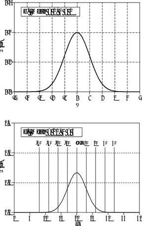
Vpp F
Vpp
F
Vpp F
Vpp
F
FIGURE 2-2
Ratio of the peak-to-peak amplitude to the standard deviation for several common waveforms. For the square wave, this ratio is 2; for the triangle wave it is 12' 3.46; for the sine wave it is 2 2' 2.83. While random noise has no exact peak-to-peak value, it is approximately 6 to 8 times the standard deviation.
a. Square Wave, Vpp = 2F
c. Sine wave, Vpp = 2 2F d. Random noise, Vpp . 6-8 F b. Triangle wave, Vpp = 12F
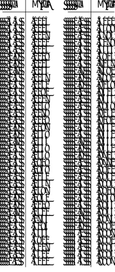
100 CALCULATION OF THE MEAN AND STANDARD DEVIATION 110 '
120 DIM X[511] 'The signal is held in X[0] to X[511]
130 N% = 512 'N% is the number of points in the signal
140 '
150 GOSUB XXXX 'Mythical subroutine that loads the signal into X[ ] 160 '
170 MEAN = 0 'Find the mean via Eq. 2-1
180 FOR I% = 0 TO N%-1 190 MEAN = MEAN + X[I%] 200 NEXT I%
210 MEAN = MEAN/N% 220 '
230 VARIANCE = 0 'Find the standard deviation via Eq. 2-2 240 FOR I% = 0 TO N%-1
250 VARIANCE = VARIANCE + ( X[I%] - MEAN )^2 260 NEXT I%
270 VARIANCE = VARIANCE/(N%-1) 280 SD = SQR(VARIANCE)
290 '
300 PRINT MEAN SD 'Print the calculated mean and standard deviation 310 '
320 END
TABLE 2-1
F
2'
1N
&
1j
N&1
i'0
x
i2&
1N
j
N&1
i'0
x
i2 EQUATION 2-3
Calculation of the standard deviation using running statistics. This equation provides the same result as Eq. 2-2, but with less round-o f f n round-o i s e a n d g r e a t e r c round-o m p u t a t i round-o n a l efficiency. The signal is expressed in terms of three accumulated parameters: N, the total number of samples; sum, the sum of these samples; and sum of squares, the sum of the squares of the samples. The mean and standard deviation are then calculated from these three accumulated parameters.
or using a simpler notation,
F
2'
1N
&
1sum of squares
&
sum
2N
in DSP. If you can't grasp one, maybe the other will help. In BASIC, the % character at the end of a variable name indicates it is an integer. All other variables are floating point. Chapter 4 discusses these variable types in detail.
This method of calculating the mean and standard deviation is adequate for many applications; however, it has two limitations. First, if the mean is much larger than the standard deviation, Eq. 2-2 involves subtracting two numbers that are very close in value. This can result in excessive round-off error in the calculations, a topic discussed in more detail in Chapter 4. Second, it is often desirable to recalculate the mean and standard deviation as new samples are acquired and added to the signal. We will call this type of calculation: running statistics. While the method of Eqs. 2-1 and 2-2 can be used for running statistics, it requires that all of the samples be involved in each new calculation. This is a very inefficient use of computational power and memory.
A solution to these problems can be found by manipulating Eqs. 2-1 and 2-2 to provide another equation for calculating the standard deviation:
While moving through the signal, a running tally is kept of three parameters: (1) the number of samples already processed, (2) the sum of these samples, and (3) the sum of the squares of the samples (that is, square the value of each sample and add the result to the accumulated value). After any number of samples have been processed, the mean and standard deviation can be efficiently calculated using only the current value of the three parameters. Table 2-2 shows a program that reports the mean and standard deviation in this manner as each new sample is taken into account. This is the method used in hand calculators to find the statistics of a sequence of numbers. Every time you enter a number and press the E (summation) key, the three
100 'MEAN AND STANDARD DEVIATION USING RUNNING STATISTICS 110 '
120 DIM X[511] 'The signal is held in X[0] to X[511]
130 '
140 GOSUB XXXX 'Mythical subroutine that loads the signal into X[ ] 150 '
160 N% = 0 'Zero the three running parameters
170 SUM = 0
180 SUMSQUARES = 0 190 '
200 FOR I% = 0 TO 511 'Loop through each sample in the signal 210 '
220 N% = N%+1 'Update the three parameters
230 SUM = SUM + X(I%)
240 SUMSQUARES = SUMSQUARES + X(I%)^2 250 '
260 MEAN = SUM/N% 'Calculate mean and standard deviation via Eq. 2-3 270 VARIANCE = (SUMSQUARES - SUM^2/N%) / (N%-1)
280 SD = SQR(VARIANCE) 290 '
300 PRINT MEAN SD 'Print the running mean and standard deviation 310 '
320 NEXT I% 330 '
340 END
TABLE 2-2
Before ending this discussion on the mean and standard deviation, two other terms need to be mentioned. In some situations, the mean describes what is being measured, while the standard deviation represents noise and other interference. In these cases, the standard deviation is not important in itself, but only in comparison to the mean. This gives rise to the term: signal-to-noise ratio (SNR), which is equal to the mean divided by the standard deviation. Another term is also used, the coefficient of variation (CV). This is defined as the standard deviation divided by the mean, multiplied by 100 percent. For example, a signal (or other group of measure values) with a CV of 2%, has an SNR of 50. Better data means a higher value for the SNR and a lower value for the CV.
Signal vs. Underlying Process
Statistics is the science of interpreting numerical data, such as acquired signals. In comparison, probability is used in DSP to understand the
processes that generate signals. Although they are closely related, the
distinction between the acquired signal and the underlying process is key to many DSP techniques.
EQUATION 2-4
Typical error in calculating the mean of an underlying process by using a finite number of samples, N. The parameter, σ , is the standard deviation.
Typical error
'
F
N
1/2will make the number of ones and zeros slightly different each time the signal is generated. The probabilities of the underlying process are constant, but the
statistics of the acquired signal change each time the experiment is repeated.
This random irregularity found in actual data is called by such names as: statistical variation, statistical fluctuation, and statistical noise.
This presents a bit of a dilemma. When you see the terms: mean and standard
deviation, how do you know if the author is referring to the statistics of an
actual signal, or the probabilities of the underlying process that created the signal? Unfortunately, the only way you can tell is by the context. This is not so for all terms used in statistics and probability. For example, the histogram
and probability mass function (discussed in the next section) are matching
concepts that are given separate names.
Now, back to Eq. 2-2, calculation of the standard deviation. As previously mentioned, this equation divides by N-1 in calculating the average of the squared deviations, rather than simply by N. To understand why this is so, imagine that you want to find the mean and standard deviation of some process that generates signals. Toward this end, you acquire a signal of N samples from the process, and calculate the mean of the signal via Eq. 2.1. You can then use this as an
estimate of the mean of the underlying process; however, you know there will
be an error due to statistical noise. In particular, for random signals, the typical error between the mean of the N points, and the mean of the underlying process, is given by:
If N is small, the statistical noise in the calculated mean will be very large. In other words, you do not have access to enough data to properly characterize the process. The larger the value of N, the smaller the expected error will become. A milestone in probability theory, the Strong Law of
Large Numbers, guarantees that the error becomes zero as N approaches
infinity.
Sample number
0 64 128 192 256 320 384 448 512
-4 -2 0 2 4 6 8
511 a. Changing mean and standard deviation
Sample number
0 64 128 192 256 320 384 448 512
-4 -2 0 2 4 6 8
511 b. Changing mean, constant standard deviation
Amplitude
Amplitude
FIGURE 2-3
Examples of signals generated from nonstationary processes. In (a), both the mean and standard deviation change. In (b), the standard deviation remains a constant value of one, while the mean changes from a value of zero to two. It is a common analysis technique to break these signals into short segments, and calculate the statistics of each segment individually.
estimate of the standard deviation of the underlying process. In other words, Eq. 2-2 is an estimate of the standard deviation of the underlying process. If we divided by N in the equation, it would provide the standard deviation of the
acquired signal.
As an illustration of these ideas, look at the signals in Fig. 2-3, and ask: are the variations in these signals a result of statistical noise, or is the underlying process changing? It probably isn't hard to convince yourself that these changes are too large for random chance, and must be related to the underlying process. Processes that change their characteristics in this manner are called nonstationary. In comparison, the signals previously presented in Fig. 2-1 were generated from a stationary process, and the variations result completely from statistical noise. Figure 2-3b illustrates a common problem with nonstationary signals: the slowly changing mean interferes with the calculation of the standard deviation. In this example, the standard deviation of the signal, over a short interval, is one. However, the standard deviation of the entire signal is 1.16. This error can be nearly eliminated by breaking the signal into short sections, and calculating the statistics for each section individually. If needed, the standard deviations for each of the sections can be averaged to produce a single value.
The Histogram, Pmf and Pdf
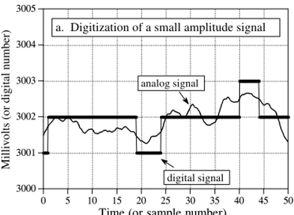
Suppose we attach an 8 bit analog-to-digital converter to a computer, and acquire 256,000 samples of some signal. As an example, Fig. 2-4a shows 128 samples that might be a part of this data set. The value of each sample will be one of 256 possibilities, 0 through 255. The histogram displays the
number of samples there are in the signal that have each of these possible
Value of sample
b. 128 point histogram
Value of sample
c. 256,000 point histogram
Sample number
Examples of histograms. Figure (a) shows 128 samples from a very long signal, with each sample being an integer between 0 and 255. Figures (b) and (c) shows histograms using 128 and 256,000 samples from the signal, respectively. As shown, the histogram is smoother when more samples are used.
EQUATION 2-5
The sum of all of the values in the histogram is equal to the number of points in the signal. In this equation, Hi is the histogram, N is the
number of points in the signal, and M is the number of points in the histogram.
N
'
j
M&1
i'0
H
iexample, there are 2 samples that have a value of 110, 8 samples that have a value of 131, 0 samples that have a value of 170, etc. We will represent the histogram by Hi, where i is an index that runs from 0 to M-1, and M is the number of possible values that each sample can take on. For instance, H50 is the number of samples that have a value of 50. Figure (c) shows the histogram of the signal using the full data set, all 256k points. As can be seen, the larger number of samples results in a much smoother appearance. Just as with the mean, the statistical noise (roughness) of the histogram is inversely proportional to the square root of the number of samples used.
From the way it is defined, the sum of all of the values in the histogram must be equal to the number of points in the signal:
EQUATION 2-6
Calculation of the mean from the histogram. This can be viewed as combining all samples having the same value into groups, and then using Eq. 2-1 on each group.
Calculation of the standard deviation from the histogram. This is the same concept as Eq. 2-2, except that all samples having the same value are operated on at once.
F
2'
1100 'CALCULATION OF THE HISTOGRAM, MEAN, AND STANDARD DEVIATION 110 '
120 DIM X%[25000] 'X%[0] to X%[25000] holds the signal being processed
130 DIM H%[255] 'H%[0] to H%[255] holds the histogram
140 N% = 25001 'Set the number of points in the signal
150 '
160 FOR I% = 0 TO 255 'Zero the histogram, so it can be used as an accumulator 170 H%[I%] = 0
180 NEXT I% 190 '
200 GOSUB XXXX 'Mythical subroutine that loads the signal into X%[ ] 210 '
220 FOR I% = 0 TO 25000 'Calculate the histogram for 25001 points 230 H%[ X%[I%] ] = H%[ X%[I%] ] + 1
240 NEXT I% 250 '
260 MEAN = 0 'Calculate the mean via Eq. 2-6
270 FOR I% = 0 TO 255
280 MEAN = MEAN + I% * H%[I%] 290 NEXT I%
300 MEAN = MEAN / N% 310 '
320 VARIANCE = 0 'Calculate the standard deviation via Eq. 2-7 330 FOR I% = 0 TO 255
340 VARIANCE = VARIANCE + H[I%] * (I%-MEAN)^2 350 NEXT I%
360 VARIANCE = VARIANCE / (N%-1) 370 SD = SQR(VARIANCE)
380 '
390 PRINT MEAN SD 'Print the calculated mean and standard deviation. 400 '
410 END
TABLE 2-3
together that have the same value. This allows the statistics to be calculated by working with a few groups, rather than a large number of individual samples. Using this approach, the mean and standard deviation are calculated from the histogram by the equations:
calculating the mean and standard deviation requires the time consuming operations of addition and multiplication. The strategy of this algorithm is to use these slow operations only on the few numbers in the histogram, not the many samples in the signal. This makes the algorithm much faster than the previously described methods. Think a factor of ten for very long signals with the calculations being performed on a general purpose computer. The notion that the acquired signal is a noisy version of the underlying process is very important; so important that some of the concepts are given different names. The histogram is what is formed from an acquired signal. The corresponding curve for the underlying process is called the probability mass function (pmf). A histogram is always calculated using a finite number of samples, while the pmf is what would be obtained with an infinite number of samples. The pmf can be estimated (inferred) from the histogram, or it may be deduced by some mathematical technique, such as in the coin flipping example.
Figure 2-5 shows an example pmf, and one of the possible histograms that could be associated with it. The key to understanding these concepts rests in the units of the vertical axis. As previously described, the vertical axis of the histogram is the number of times that a particular value occurs in the signal. The vertical axis of the pmf contains similar information, except expressed on a fractional
basis. In other words, each value in the histogram is divided by the total
number of samples to approximate the pmf. This means that each value in the pmf must be between zero and one, and that the sum of all of the values in the pmf will be equal to one.
The pmf is important because it describes the probability that a certain value will be generated. For example, imagine a signal with the pmf of Fig. 2-5b, such as previously shown in Fig. 2-4a. What is the probability that a sample taken from this signal will have a value of 120? Figure 2-5b provides the answer, 0.03, or about 1 chance in 34. What is the probability that a randomly chosen sample will have a value greater than 150? Adding up the values in the pmf for: 151, 152, 153,@@@, 255, provides the answer, 0.0122, or about 1 chance in 82. Thus, the signal would be expected to have a value exceeding 150 on an average of every 82 points. What is the probability that any one sample will be between 0 and 255? Summing all of the values in the histogram produces the probability of 1.00, a certainty that this will occur.
Value of sample
c. Probability Density Function (pdf)
Value of sample
b. Probability Mass Function (pmf)
Probability of occurence
Probability density
Number of occurences
FIGURE 2-5
The relationship between (a) the histogram, (b) the probability mass function (pmf), and (c) the probability density function (pdf). The histogram is calculated from a finite number of samples. The pmf describes the probabilities of the underlying process. The pdf is similar to the pmf, but is used with continuous rather than discrete signals. Even though the vertical axis of (b) and (c) have the same values (0 to 0.06), this is only a coincidence of this example. The amplitude of these three curves is determined by: (a) the sum of the values in the histogram being equal to the number of samples in the signal; (b) the sum of the values in the pmf being equal to one, and (c) the area under the pdf curve being equal to one.
signal is shown by the markers in Fig. 2-5b. Similarly, the pdf of the analog signal is shown by the continuous line in (c), indicating the signal can take on a continuous range of values, such as the voltage in an electronic circuit.
The vertical axis of the pdf is in units of probability density, rather than just probability. For example, a pdf of 0.03 at 120.5 does not mean that the a voltage of 120.5 millivolts will occur 3% of the time. In fact, the probability of the continuous signal being exactly 120.5 millivolts is infinitesimally small. This is because there are an infinite number of possible values that the signal needs to divide its time between: 120.49997, 120.49998, 120.49999, etc. The chance that the signal happens to be exactly 120.50000þ is very remote indeed!
To calculate a probability, the probability density is multiplied by a range of values. For example, the probability that the signal, at any given instant, will be between the values of 120 and 121 is: 121&120 × 0.03' 0.03. The probability that the signal will be between 120.4 and 120.5 is: , etc. If the pdf is not constant over the range of 120.5&120.4 × 0.03'0.003
Time (or other variable)
0 16 32 48 64 80 96 112 128
-2 -1 0 1 2
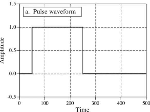
a. Square wave
127
FIGURE 2-6
Three common waveforms and their probability density functions. As in these examples, the pdf graph is often rotated one-quarter turn and placed at the side of the signal it describes. The pdf of a square wave, shown in (a), consists of two infinitesimally narrow spikes, corresponding to the signal only having two possible values. The pdf of the triangle wave, (b), has a constant value over a range, and is often called a uniform distribution. The pdf of random noise, as in (c), is the most interesting of all, a bell shaped curve known as a Gaussian.
Time (or other variable)
0 16 32 48 64 80 96 112 128
-2 -1 0 1 2
127
pdf b. Triangle wave
Time (or other variable)
0 16 32 48 64 80 96 112 128
-2 -1 0 1 2
127
c. Random noise
Amplitude
Amplitude
Amplitude
curve, the integral from &4 to %4, will always be equal to one. This is analogous to the sum of all of the pmf values being equal to one, and the sum of all of the histogram values being equal to N.
100 'CALCULATION OF BINNED HISTOGRAM 110 '
120 DIM X[25000] 'X[0] to X[25000] holds the floating point signal,
130 ' 'with each sample being in the range: 0.0 to 10.0
140 DIM H%[999] 'H%[0] to H%[999] holds the binned histogram
150 '
160 FOR I% = 0 TO 999 'Zero the binned histogram for use as an accumulator 170 H%[I%] = 0
180 NEXT I% 190 '
200 GOSUB XXXX 'Mythical subroutine that loads the signal into X%[ ] 210 '
220 FOR I% = 0 TO 25000 'Calculate the binned histogram for 25001 points 230 BINNUM% = INT( X[I%] * .01 )
240 H%[ BINNUM%] = H%[ BINNUM%] + 1 250 NEXT I%
260 ' 270 END
TABLE 2-4
engineers. Figure 2-6 shows three continuous waveforms and their pdfs. If these were discrete signals, signified by changing the horizontal axis labeling to "sample number," pmfs would be used.
A problem occurs in calculating the histogram when the number of levels each sample can take on is much larger than the number of samples in the signal. This is always true for signals represented in floating point
notation, where each sample is stored as a fractional value. For example, integer representation might require the sample value to be 3 or 4, while floating point allows millions of possible fractional values between 3 and 4. The previously described approach for calculating the histogram involves counting the number of samples that have each of the possible quantization levels. This is not possible with floating point data because there are
billions of possible levels that would have to be taken into account. Even
worse, nearly all of these possible levels would have no samples that correspond to them. For example, imagine a 10,000 sample signal, with each sample having one billion possible values. The conventional histogram would consist of one billion data points, with all but about 10,000 of them having a value of zero.
The solution to these problems is a technique called binning. This is done by arbitrarily selecting the length of the histogram to be some convenient number, such as 1000 points, often called bins. The value of each bin represent the total number of samples in the signal that have a value within
a certain range. For example, imagine a floating point signal that contains
![Figure 6-2 shows the notation when convolution is used with linear systems. An input signal, x [n] , enters a linear system with an impulse response, h [n] , resulting in an output signal, y [n]](https://thumb-ap.123doks.com/thumbv2/123dok/4032092.1975512/123.783.381.686.839.929/figure-notation-convolution-systems-linear-impulse-response-resulting.webp)
![Figure 6-5 shows a simple convolution problem: a 9 point input signal, x [n] , is passed through a system with a 4 point impulse response, h [n] , resulting in a 9 % 4 & 1 ' 12 point output signal, y [n]](https://thumb-ap.123doks.com/thumbv2/123dok/4032092.1975512/126.783.102.676.710.889/figure-convolution-problem-signal-impulse-response-resulting-output.webp)

