Afterword
When writing about data compression, I am haunted by the idea that many of the techniques discussed in this book have been patented by their inventors or others. The knowledge that a data compression algorithm can effectively be taken out of the hands of programmers through the use of so-called “intellectual property” law seems contrary to the basic principles that led me and many others into this profession.
I have yet to see any evidence that applying patents to software advances that art or protects the rights of inventors. Several companies continue to collect royalties on patents long after their inventors have moved onto bigger and better thing with other companies. Have the patent-holders done anything notable other than collect royalties? Have they advanced the art of computer science?
Making a software product into a commercial success requires innovation, good design, high-quality documentation, and listening to customers. These are things that nobody can steal from you. On the other hand, a mountain of patents can’t keep you from letting these things slip away through
inattention or complacency. This lesson seems to be lost on those who traffic in intellectual property “portfolios.”
What can you do? First, don’t patent your own work, and discourage your peers from doing so. Work on improving your products, not erecting legal obstacles to competition. Secondly, lobby for change. This means change within your company, those you do business with, and most importantly, within the federal government. Write to your congressman and your senator. Write to the ACM. Write to the House Subcommittee on Intellectual Property. And finally, you can join me by becoming a member of the League for Programming Freedom. Write for more information:
League For Programming Freedom 1 Kendall Square #143
P.O. Box 9171
I concluded, we kinotropists must be numbered among Britain's most adept programmers of Enginery of any sort, and virtually all advances on the compression of data have originated as kinotropic applications.
At this point, he interrupted again, asking if I had indeed said "the compression of data," and was I familiar with the term "algorithmic compression"? I assured him I was.
The Difference Engine
William Gibson and Bruce Sterling
Why This Book Is For You
If you want to learn how programs like PKZIP and LHarc work, this book is for you. The
compression techniques used in these programs are described in detail, accompanied by working code. After reading this book, even the novice C programmer will be able to write a complete compression/archiving program that can be ported to virtually any operating system or hardware platform.
If you want to include data compression in other programs you write, this book will become an invaluable tool. It contains dozens of working programs with C code that can easily be added to your applications. In-depth discussions of various compression methods will help you make intelligent decisions when creating programs that use data compression.
If you want to learn why lossy compression of graphics is the key factor in enabling the multimedia revolution, you need this book. DCT-based compression like that used by the JPEG algorithm is described in detail. The cutting edge technology of fractal compression is explained in useful terms, instead of the purly theoretical. Working programs let you experiment with these fascinating new technologies.
(Imprint: M & T Books)
(Publisher: IDG Books Worldwide, Inc.) Author: Mark Nelson
ISBN: 1558514341
Afterword
Why This Book Is For You
Chapter 1—Introduction to Data Compression
The Audience Why C? Which C?
Issues in Writing Portable C Keeping Score
The Structure
Chapter 2—The Data-Compression Lexicon, with a History
The Two Kingdoms
Data Compression = Modeling + Coding The Dawn Age
Coding
An Improvement Modeling
Statistical Modeling Dictionary Schemes Ziv and Lempel
LZ77 LZ78
Lossy Compression Programs to Know
Chapter 3—The Dawn Age: Minimum Redundancy Coding
The Shannon-Fano Algorithm The Huffman Algorithm Huffman in C
BITIO.C
A Reminder about Prototypes MAIN-C.C AND MAIN-E.C
MAIN-C.C ERRHAND.C Into the Huffman Code
Counting the Symbols Saving the Counts Building the Tree Using the Tree The Compression Code Putting It All Together
Performance
Chapter 4—A Significant Improvement: Adaptive Huffman Coding
Adaptive Coding
The Algorithm An Enhancement The Escape Code The Overflow Problem A Rescaling Bonus The Code
Initialization of the Array The Compress Main Program The Expand Main Program Encoding the Symbol Updating the Tree Decoding the Symbol The Code
Chapter 5—Huffman One Better: Arithmetic Coding
Difficulties
Arithmetic Coding: A Step Forward Practical Matters
A Complication Decoding
Where’s the Beef? The Code
The Compression Program The Expansion Program Initializing the Model Reading the Model Initializing the Encoder The Encoding Process Flushing the Encoder The Decoding Process Summary
Code
Chapter 6—Statistical Modeling
Higher-Order Modeling Finite Context Modeling Adaptive Modeling
A Simple Example
Using the Escape Code as a Fallback Improvements
Highest-Order Modeling Updating the Model Escape Probabilities Scoreboarding Data Structures
The Finishing Touches: Tables –1 and –2 Model Flushing
Implementation Conclusions
Enhancement ARITH-N Listing
Chapter 7—Dictionary-Based Compression
Static vs. Adaptive Adaptive Methods
A Representative Example Israeli Roots
History
ARC: The Father of MS-DOS Dictionary Compression Dictionary Compression: Where It Shows Up Danger Ahead—Patents
Conclusion
Chapter 8—Sliding Window Compression
The Algorithm
Problems with LZ77 An Encoding Problem LZSS Compression
Data Structures A Balancing Act
Greedy vs. Best Possible The Code
Constants and Macros Global Variables The Compression Code
Initialization The Main Loop The Exit Code AddString() DeleteString()
Binary Tree Support Routines The Expansion Routine
Improvements The Code
Chapter 9—LZ78 Compression
Can LZ77 Improve? Enter LZ78
LZ78 Details
LZ78 Implementation An Effective Variant
Decompression The Catch
LZW Implementation
Tree Maintenance and Navigation Compression
Decompression The Code Improvements Patents
Chapter 10—Speech Compression
Digital Audio Concepts Fundamentals Sampling Variables PC-Based Sound
Problems and Results Lossy Compression Silence Compression Companding
Other Techniques
Chapter 11—Lossy Graphics Compression
Enter Compression
Statistical and Dictionary Compression Methods Lossy Compression
Differential Modulation Adaptive Coding
A Standard That Works: JPEG JPEG Compression
The Discrete Cosine Transform DCT Specifics
Why Bother?
Implementing the DCT Matrix Multiplication Continued Improvements
Output of the DCT Quantization
Selecting a Quantization Matrix Coding
The Zig-Zag Sequence Entropy Encoding What About Color? The Sample Program
Input Format The Code Initialization
The Forward DCT Routine WriteDCTData()
OutputCode() File Expansion ReadDCTData() Input DCT Codes The Inverse DCT The Complete Code Listing Support Programs
Some Compression Results
Chapter 12—An Archiving Package
CAR and CARMAN
The CARMAN Command Set The CAR File
The Header
Storing the Header The Header CRC
Command-Line Processing Generating the File List
Opening the Archive Files The Main Processing Loop
File Insertion File Extraction Cleanup
The Code
Chapter 13—Fractal Image Compression
A brief history of fractal image compression What is an Iterated Function System?
Basic IFS mathematics
Image compression with Iterated Function Systems
Image compression with Partitioned Iterated Function Systems Fractal image decoding
Resolution independence The sample program
The main compression module Initialization
Domain classification Image partitioning
Finding optimal affine maps The decompression module The complete code listing
Some Compression Results Patents
Chapter 1
Introduction to Data Compression
The primary purpose of this book is to explain various data-compression techniques using the C programming language. Data compression seeks to reduce the number of bits used to store or transmit information. It encompasses a wide variety of software and hardware compression techniques which can be so unlike one another that they have little in common except that they compress data. The LZW algorithm used in the Compuserve GIF specification, for example, has virtually nothing in common with the CCITT G.721 specification used to compress digitized voice over phone lines.
This book will not take a comprehensive look at every variety of data compression. The field has grown in the last 25 years to a point where this is simply not possible. What this book will cover are the various types of data compression commonly used on personal and midsized computers,
including compression of binary programs, data, sound, and graphics.
Furthermore, this book will either ignore or only lightly cover data-compression techniques that rely on hardware for practical use or that require hardware applications. Many of today’s
voice-compression schemes were designed for the worldwide fixed-bandwidth digital telecommunications networks. These compression schemes are intellectually interesting, but they require a specific type of hardware tuned to the fixed bandwidth of the communications channel. Different algorithms that don’t have to meet this requirement are used to compress digitized voice on a PC, and these
algorithms generally offer better performance.
Some of the most interesting areas in data compression today, however, do concern compression techniques just becoming possible with new and more powerful hardware. Lossy image
compression, like that used in multimedia systems, for example, can now be implemented on standard desktop platforms. This book will cover practical ways to both experiment with and implement some of the algorithms used in these techniques.
The Audience
You will need basic programming skills to adequately discuss data-compression code. The ability to follow block-structured code, such as C or Pascal, is a requirement. In addition, understanding computer architecture well enough to follow bit-oriented operations, such as shifting, logical ORing and ANDing, and so on, will be essential.
This does not mean that you need to be a C guru for this book to be worthwhile. You don’t even have to be a programmer. But the ability to follow code will be essential, because the concepts discussed here will be illustrated with portable C programs. The C code in this book has been written with an eye toward simplicity in the hopes that C novices will still be able to follow the programs. We will avoid the more esoteric constructs of C, but the code will be working tested C—no pseudocode or English.
Why C?
If pseudocode is unsatisfactory, the next best choice is to use a conventional programming language. Though hundreds of choices are available, C seems the best choice for this type of book for several good reasons. First, in many respects C has become the lingua franca of programmers. That C compilers support computers ranging from a lowly 8051 microcontroller to supercomputers capable of 100 million instructions per second (MIPS) has had much to do with this. It doesn’t mean that C is the language of choice for all programmers. What it does mean is that most programmers should have a C compiler available for their machines, and most are probably regularly exposed to C code. Because of this, many programmers who use other languages can still manage to code in C, and even more can at least read C.
A second reason for using C is that it is a language without too many surprises. The few constructs it uses as basic language elements are easily translated to other languages. So a data-compression program that is illustrated using C can be converted to a working Pascal program through a relatively straightforward translation procedure. Even assembly-language programmers should find the process relatively painless.
Perhaps the most important reason for using C is simply one of efficiency. C is often thought of as a high-level assembly language, since it allows programmers to get close to the hardware. Despite the increasing optimization found in recent C compilers, it is not likely that C will ever exceed the speed or size possible in hand-coded assembly language. That flaw is offset, however, by the ability to easily port C code to other machines. So for a book of this type, C is probably the most efficient choice.
Which C?
Despite being advertised as a “portable” language, a C program that compiles and executes on a given machine is not guaranteed to run on any other. It may not even compile using a different compiler on the same machine. The important thing to remember is not that C is portable, but that it
can be portable. The code for this book has been written to be portable, and it compiles and runs cleanly using several compilers and environments. The compilers/environments used here include:
• Microsoft Visual C++ 1.5, MS-DOS 5.0/6.22 • Borland C++ 4.0-4.5, MS-DOS 5.0/6.22 • Symantec C++ 6.0-7.0, MS-DOS 5.0/6.22
• Interactive Unix System 3.2 with the portable C compiler • Solaris 2.4 with SunSoft compiler
• Linux 1.1 with the GNU C compiler
Issues in Writing Portable C
One important portability issue is library function calls. Though the C programming language was fairly well defined by the original K&R book (Brian W. Kernighan and Dennis M. Ritchie, The C Programming Language [Englewood Cliffs, NJ.: Prentice-Hall, 1978]), the run-time library implementation was left totally up to the whims of the implementor. Fortunately, the American National Standards Institute was able to complete the C language specification in 1990, and the result was published as ANSI standard XJ11.34. This standard not only expanded and pinned down the original K&R language specification, but it also took on the definition of a standard C run-time library. This makes it much easier to write code that works the same way from machine to machine. The code in this book will be written with the intention of using only ANSI C library calls.
Compiler-dependent extensions to either the language or the library will be avoided wherever possible.
sizes of the basic data types and dealing with noncompliant compilers. The majority of data-type conflicts arise when switching between 16- and 32-bit machines.
Fortunately, it is fairly easy to manage the change between 16- and 32-bit machines. Though the basic integer data type switches between 16- and 32-bits, both machines have a 16-bit “short int” data type. Once again, a “long int” is generally 32 bits on both machines. So in cases where the size of an integer clearly matters, it can be pinned down to either 16-or 32-bits with the appropriate declaration.
On the vast majority of machines used in the world today, the C compiler implementation of the “char” data type is 8 bits wide. In this book, we will gloss over the possibility that any other size exists and stick with 8-bit characters. In general, porting a program shown here to a machine with an unusual char size is not too difficult, but spending too much time on it will obscure the important point of the programs here, which is data compression.
The final issue to deal with when writing portable code is the problem of noncompliant compilers. In the MS-DOS world, most C compilers undergo major releases and upgrades every two years or so. This means that most compiler vendors have been able to release new versions of their compilers that now conform closely to the ANSI C standard. But this is not the case for users of many other operating systems. In particular, UNIX users will frequently be using a C compiler which came with their system and which conforms to the older K&R language definition. While the ANSI C
committee went to great lengths to make ANSI C upwardly compatible from K&R C, we need to watch out for a few problems.
The first problem lies in the use of function prototypes. Under K&R C, function prototypes were generally used only when necessary. The compiler assumed that any unseen function returned an integer, and it accepted this without complaint. If a function returned something unusual—a pointer or a long, for instance—the programmer would write a function prototype to inform the compiler.
long locate_string();
Here, the prototype told the compiler to generate code that assumes that the function returned a long instead of an int. Function prototypes didn’t have much more use than that. Because of this, many C programmers working under a K&R regime made little or no use of function prototypes, and their appearance in a program was something of an oddity.
While the ANSI C committee tried not to alter the basic nature of C, they were unable to pass up the potential improvements to the language that were possible through the expansion of the prototyping facility. Under ANSI C, a function prototype defines not only the return type of a function, but also the type of all the arguments as well. The function shown earlier, for example, might have the following prototype with an ANSI C compiler:
long locate_string( FILE *input_file, char *string );
This lets the compiler generate the correct code for the return type and check for the correct type and number of arguments as well. Since passing the wrong type or number of arguments to a function is a major source of programmer error in C, the committee correctly assumed that allowing this form of type checking constituted a step forward for C.
Under many ANSI C compilers, use of full ANSI function prototypes is strongly encouraged. In fact, many compilers will generate warning messages when a function is used without previously
The solution to this dilemma is not pretty, but it works. Under ANSI C, the predefined macro ___STDC___ is always defined to indicate that the code is being compiled through a presumably ANSI-compliant compiler. We can let the preprocessor turn certain sections of our header files on or off, depending on whether we are using a noncompliant compiler or not. A header file containing the prototypes for a bit-oriented package, for example, might look something like this:
#ifdef ___STDC___
FILE *open_bitstream( char *file_name, char *mode ); void close_bitstream( FILE *bitstream );
int read_bit( FILE*bitstream );
int write_bit( FILE *bitstream, int bit );
#else
FILE *open_bitstream(); void close_bitstream(); int read_bit();
int write_bit();
#endif
The preprocessor directives don’t contribute much to the look of the code, but they are a necessary part of writing portable programs. Since the programs in this book are supposed to be compiled with the compiler set to its maximum possible warning level, a few “#ifdef” statements will be part of the package.
A second problem with the K&R family of C compilers lies in the actual function body. Under K&R C, a particular function might have a definition like the one below.
int foo( c ) char c; {
/* Function body */ }
The same function written using an ANSI C function body would look like this:
int foo( char c ) {
/* Function body */ }
These two functions may look the same, but ANSI C rules require that they be treated differently. The K&R function body will have the compiler “promote” the character argument to an integer before using it in the function body, but the ANSI C function body will leave it as a character. Promoting one integral type to another lets lots of sneaky problems slip into seemingly well-written code, and the stricter compilers will issue warnings when they detect a problem of this nature.
Since K&R compilers will not accept the second form of a function body, be careful when defining character arguments to functions. Unfortunately, the solutions are once again either to not use character arguments or to resort to more of the ugly “#ifdef” preprocessor baggage.
Keeping Score
in relationship to the sample compression files used in the February 1991 Dr. Dobb’s Journal compression contest. These files consist of about 6 megabytes of data broken down into three
roughly equal categories. The first category is text, consisting of manuscripts, programs, memos, and other readable files. The second category consists of binary data, including database files, executable files, and spreadsheet data. The third category consists of graphics files stored in raw screen-dump formats.
The programs created and discussed in this book will be judged by three rough measures of
performance. The first will be the amount of memory consumed by the program during compression; this number will be approximated as well as it can be. The second will be the amount of time the program takes to compress the entire Dr. Dobb’s dataset. The third will be the compression ratio of the entire set.
Different people use different formulas to calculate compression ratios. Some prefer bits/bytes. Other use ratios, such as 2:1 or 3:1 (advertising people seem to like this format). In this book, we will use a simple compression-percentage formula:
( 1 - ( compressed_size / raw_size ) ) * 100
This means that a file that doesn’t change at all when compressed will have a compression ratio of 0 percent. A file compressed down to one-third of its original size will have a compression ratio of 67 percent. A file that shrinks down to 0 bytes (!) will have a compression ratio of 100 percent.
This way of measuring compression may not be perfect, but it shows perfection at 100 percent and total failure at 0 percent. In fact, a file that goes through a compression program and comes out larger will show a negative compression ratio.
The Structure
This book consists of thirteen chapters and a floppy disk. The organization roughly parallels the historical progression of data compression, starting in the “dawn age” around 1950 and working up to the present.
Chapter 2 is a reference chapter which attempts to establish the fundamental data-compression lexicon. It discusses the birth of information theory, and it introduces a series of concepts, terms, buzzwords, and theories used over and over in the rest of the book. Even if you are a
data-compression novice, mastery of chapter 2 will bring you up to the “cocktail party” level of
information, meaning that you will be able to carry on an intelligent-sounding conversation about data compression even if you don’t fully understand its intricacies.
Chapter 3 discusses the birth of data compression, starting with variable-length bit coding. The development of Shannon-Fano coding and Huffman coding represented the birth of both data compression and information theory. These coding methods are still in wide use today. In addition, chapter 3 discusses the difference between modeling and coding—the two faces of the
data-compression coin.
Huffman coding has to use an integral number of bits for each code, which is usually slightly less than optimal. A more recent innovation, arithmetic coding, uses a fractional number of bits per code, allowing it to incrementally improve compression performance. Chapter 5 explains how this recent innovation works, and it shows how to integrate an arithmetic coder with a statistical model.
Chapter 6 discusses statistical modeling. Whether using Huffman coding, adaptive Huffman coding, or arithmetic coding, it is still necessary to have a statistical model to drive the coder. This chapter shows some of the interesting techniques used to implement powerful models using limited memory resources.
Dictionary compression methods take a completely different approach to compression from the techniques discussed in the previous four chapters. Chapter 7 provides an overview of these compression methods, which represent strings of characters with single codes. Dictionary methods have become the de facto standard for general-purpose data compression on small computers due to their high-performance compression combined with reasonable memory requirements.
The fathers of dictionary-based compression, Ziv and Lempel published a paper in 1977 proposing a sliding dictionary methods of data compression which has become very popular. Chapter 8 looks at recent adaptations of LZ77 compression used in popular archiving programs such as PKZIP.
Chapter 9 takes detailed look at one of the first widely popular dictionary-based compression methods: LZW compression. LZW is the compression method used in the UNIX COMPRESS program and in earlier versions of the MS-DOS ARC program. This chapter also takes a look at the foundation of LZW compression, published in 1978 by Ziv and Lempel.
All of the compression techniques discussed through chapter 9 are “lossless.” Lossy methods can be used on speech and graphics, and they are capable of achieving dramatically higher compression ratios. Chapter 10 shows how lossy compression can be used on digitized sound data which techniques like linear predictive coding and adaptive PCM.
Chapter 11 discusses lossy compression techniques applied to computer graphics. The industry is standardizing rapidly on the JPEG standard for compressing graphical images. The techniques used in the JPEG standard will be presented in this chapter.
Chapter 12 describes how to put it all together into an archive program. A general-purpose archiving program should be able to compress and decompress files while keeping track of files names, dates, attributes, compression ratios, and compression methods. An archive format should ideally be portable to different types of computers. A sample archive program is developed, which applies the techniques used in previous chapters to put together a complete program.
Chapter 2
The Data-Compression Lexicon, with a History
Like any other scientific or engineering discipline, data compression has a vocabulary that at first seem overwhelmingly strange to an outsider. Terms like Lempel-Ziv compression, arithmetic coding, and statistical modeling get tossed around with reckless abandon.
While the list of buzzwords is long enough to merit a glossary, mastering them is not as daunting a project as it may first seem. With a bit of study and a few notes, any programmer should hold his or her own at a cocktail-party argument over data-compression techniques.
The Two Kingdoms
Data-compression techniques can be divided into two major families; lossy and lossless. Lossy data compression concedes a certain loss of accuracy in exchange for greatly increased compression. Lossy compression proves effective when applied to graphics images and digitized voice. By their very nature, these digitized representations of analog phenomena are not perfect to begin with, so the idea of output and input not matching exactly is a little more acceptable. Most lossy compression techniques can be adjusted to different quality levels, gaining higher accuracy in exchange for less effective compression. Until recently, lossy compression has been primarily implemented using dedicated hardware. In the past few years, powerful lossy-compression programs have been moved to desktop CPUs, but even so the field is still dominated by hardware implementations.
Lossless compression consists of those techniques guaranteed to generate an exact duplicate of the input data stream after a compress/expand cycle. This is the type of compression used when storing database records, spreadsheets, or word processing files. In these applications, the loss of even a single bit could be catastrophic. Most techniques discussed in this book will be lossless.
Data Compression = Modeling + Coding
In general, data compression consists of taking a stream of symbols and transforming them into codes. If the compression is effective, the resulting stream of codes will be smaller than the original symbols. The decision to output a certain code for a certain symbol or set of symbols is based on a model. The model is simply a collection of data and rules used to process input symbols and determine which code(s) to output. A program uses the model to accurately define the probabilities for each symbol and the coder to produce an appropriate code based on those probabilities.
Modeling and coding are two distinctly different things. People frequently use the term coding to refer to the entire data-compression process instead of just a single component of that process. You will hear the phrases “Huffman coding” or “Run-Length Encoding,” for example, to describe a data-compression technique, when in fact they are just coding methods used in conjunction with a model to compress data.
Using the example of Huffman coding, a breakdown of the compression process looks something like this:
In the case of Huffman coding, the actual output of the encoder is determined by a set of probabilities. When using this type of coding, a symbol that has a very high probability of
occurrence generates a code with very few bits. A symbol with a low probability generates a code with a larger number of bits.
We think of the model and the program’s coding process as different because of the countless ways to model data, all of which can use the same coding process to produce their output. A simple program using Huffman coding, for example, would use a model that gave the raw probability of each symbol occurring anywhere in the input stream. A more sophisticated program might calculate the probability based on the last 10 symbols in the input stream. Even though both programs use Huffman coding to produce their output, their compression ratios would probably be radically different.
So when the topic of coding methods comes up at your next cocktail party, be alert for statements like “Huffman coding in general doesn’t produce very good compression ratios.” This would be your perfect opportunity to respond with “That’s like saying Converse sneakers don’t go very fast. I always thought the leg power of the runner had a lot to do with it.” If the conversation has already dropped to the point where you are discussing data compression, this might even go over as a real demonstration of wit.
The Dawn Age
Data compression is perhaps the fundamental expression of Information Theory. Information Theory is a branch of mathematics that had its genesis in the late 1940s with the work of Claude Shannon at Bell Labs. It concerns itself with various questions about information, including different ways of storing and communicating messages.
Data compression enters into the field of Information Theory because of its concern with
redundancy. Redundant information in a message takes extra bit to encode, and if we can get rid of that extra information, we will have reduced the size of the message.
Information Theory uses the term entropy as a measure of how much information is encoded in a message. The word entropy was borrowed from thermodynamics, and it has a similar meaning. The higher the entropy of a message, the more information it contains. The entropy of a symbol is defined as the negative logarithm of its probability. To determine the information content of a message in bits, we express the entropy using the base 2 logarithm:
Number of bits = - Log base 2 (probability)
The entropy of an entire message is simply the sum of the entropy of all individual symbols.
Entropy fits with data compression in its determination of how many bits of information are actually present in a message. If the probability of the character ‘e’ appearing in this manuscript is 1/16, for example, the information content of the character is four bits. So the character string “eeeee” has a total content of 20 bits. If we are using standard 8-bit ASCII characters to encode this message, we are actually using 40 bits. The difference between the 20 bits of entropy and the 40 bits used to encode the message is where the potential for data compression arises.
How probabilities change can be seen clearly when using different orders with a statistical model. A statistical model tracks the probability of a symbol based on what symbols appeared previously in the input stream. The order of the model determines how many previous symbols are taken into account. An order-0 model, for example, won’t look at previous characters. An order-1 model looks at the one previous character, and so on.
The different order models can yield drastically different probabilities for a character. The letter ‘u’ under an order-0 model, for example, may have only a 1 percent probability of occurrence. But under an order-1 model, if the previous character was ‘q,’ the ‘u’ may have a 95 percent probability.
This seemingly unstable notion of a character’s probability proves troublesome for many people. They prefer that a character have a fixed “true” probability that told what the chances of its “really” occurring are. Claude Shannon attempted to determine the true information content of the English language with a “party game” experiment. He would uncover a message concealed from his audience a single character at a time. The audience guessed what the next character would be, one guess at a time, until they got it right. Shannon could then determine the entropy of the message as a whole by taking the logarithm of the guess count. Other researchers have done more experiments using similar techniques.
While these experiments are useful, they don’t circumvent the notion that a symbol’s probability depends on the model. The difference with these experiments is that the model is the one kept inside the human brain. This may be one of the best models available, but it is still a model, not an absolute truth.
In order to compress data well, we need to select models that predict symbols with high probabilities. A symbol that has a high probability has a low information content and will need fewer bits to
encode. Once the model is producing high probabilities, the next step is to encode the symbols using an appropriate number of bits.
Coding
Once Information Theory had advanced to where the number of bits of information in a symbol could be determined, the next step was to develop new methods for encoding information. To compress data, we need to encode symbols with exactly the number of bits of information the symbol contains. If the character ‘e’ only gives us four bits of information, then it should be coded with exactly four bits. If ‘x’ contains twelve bits, it should be coded with twelve bits.
By encoding characters using EBCDIC or ASCII, we clearly aren’t going to be very close to an optimum method. Since every character is encoded using the same number of bits, we introduce lots of error in both directions, with most of the codes in a message being too long and some being too short.
Solving this coding problem in a reasonable manner was one of the first problems tackled by practitioners of Information Theory. Two approaches that worked well were Shannon-Fano coding and Huffman coding—two different ways of generating variable-length codes when given a probability table for a given set of symbols.
Huffman coding, named for its inventor D.A. Huffman, achieves the minimum amount of
redundancy possible in a fixed set of variable-length codes. This doesn’t mean that Huffman coding is an optimal coding method. It means that it provides the best approximation for coding symbols when using fixed-width codes.
each code. If the entropy of a given character is 2.5 bits, the Huffman code for that character must be either 2 or 3 bits, not 2.5. Because of this, Huffman coding can’t be considered an optimal coding method, but it is the best approximation that uses fixed codes with an integral number of bits. Here is a sample of Huffman codes:
An Improvement
Though Huffman coding is inefficient due to using an integral number of bits per code, it is relatively easy to implement and very economical for both coding and decoding. Huffman first published his paper on coding in 1952, and it instantly became the most-cited paper in Information Theory. It probably still is. Huffman’s original work spawned numerous minor variations, and it dominated the coding world till the early 1980s.
As the cost of CPU cycles went down, new possibilities for more efficient coding techniques emerged. One in particular, arithmetic coding, is a viable successor to Huffman coding.
Arithmetic coding is somewhat more complicated in both concept and implementation than standard variable-width codes. It does not produce a single code for each symbol. Instead, it produces a code for an entire message. Each symbol added to the message incrementally modifies the output code. This is an improvement because the net effect of each input symbol on the output code can be a fractional number of bits instead of an integral number. So if the entropy for character ‘e’ is 2.5 bits, it is possible to add exactly 2.5 bits to the output code.
An example of why this can be more effective is shown in the following table, the analysis of an imaginary message. In it, Huffman coding would yield a total message length of 89 bits, but arithmetic coding would approach the true information content of the message, or 83.56 bits. The difference in the two messages works out to approximately 6 percent. Here are some sample message probabilities:
Symbol Huffman Code
E 100
T 101
A 1100
I 11010
…
X 01101111
Q 01101110001
Z 01101110000
Symbol Number of
Occurrences
Information Content
Huffman Code Bit Count
Total Bits Huffman Coding
Total Bits Arithmetic Coding
E 20 1.26 bits 1 bits 20 25.2
A 20 1.26 bits 2 bits 40 25.2
The problem with Huffman coding in the above message is that it can’t create codes with the exact information content required. In most cases it is a little above or a little below, leading to deviations from the optimum. But arithmetic coding gets to within a fraction of a percent of the actual
information content, resulting in more accurate coding.
Arithmetic coding requires more CPU power than was available until recently. Even now it will generally suffer from a significant speed disadvantage when compared to older coding methods. But the gains from switching to this method are significant enough to ensure that arithmetic coding will be the coding method of choice when the cost of storing or sending information is high enough.
Modeling
If we use a an automotive metaphor for data compression, coding would be the wheels, but modeling would be the engine. Regardless of the efficiency of the coder, if it doesn’t have a model feeding it good probabilities, it won’t compress data.
Lossless data compression is generally implemented using one of two different types of modeling: statistical or dictionary-based. Statistical modeling reads in and encodes a single symbol at a time using the probability of that character’s appearance. Dictionary-based modeling uses a single code to replace strings of symbols. In dictionary-based modeling, the coding problem is reduced in
significance, leaving the model supremely important.
Statistical Modeling
The simplest forms of statistical modeling use a static table of probabilities. In the earliest days of information theory, the CPU cost of analyzing data and building a Huffman tree was considered significant, so it wasn’t frequently performed. Instead, representative blocks of data were analyzed once, giving a table of character-frequency counts. Huffman encoding/decoding trees were then built and stored. Compression programs had access to this static model and would compress data using it.
But using a universal static model has limitations. If an input stream doesn’t match well with the previously accumulated statistics, the compression ratio will be degraded—possibly to the point where the output stream becomes larger than the input stream. The next obvious enhancement is to build a statistics table for every unique input stream.
Building a static Huffman table for each file to be compressed has its advantages. The table is uniquely adapted to that particular file, so it should give better compression than a universal table. But there is additional overhead since the table (or the statistics used to build the table) has to be passed to the decoder ahead of the compressed code stream.
For an order-0 compression table, the actual statistics used to create the table may take up as little as 256 bytes—not a very large amount of overhead. But trying to achieve better compression through use of a higher order table will make the statistics that need to be passed to the decoder grow at an alarming rate. Just moving to an order 1 model can boost the statistics table from 256 to 65,536 bytes. Though compression ratios will undoubtedly improve when moving to order-1, the overhead of passing the statistics table will probably wipe out any gains.
For this reason, compression research in the last 10 years has concentrated on adaptive models.
Y 3 4.00 bits 4 bits 12 12.0
Z 2 4.58 bits 4 bits 8 9.16
When using an adaptive model, data does not have to be scanned once before coding in order to generate statistics. Instead, the statistics are continually modified as new characters are read in and coded. The general flow of a program using an adaptive model looks something like that shown in Figures 2.2 and 2.3.
Figure 2.2 General Adaptive Compression.
Figure 2.3 General Adaptive Decompression.
The important point in making this system work is that the box labeled “Update Model” has to work exactly the same way for both the compression and decompression programs. After each character (or group of characters) is read in, it is encoded or decoded. Only after the encoding or decoding is complete can the model be updated to take into account the most recent symbol or group of symbols.
One problem with adaptive models is that they start knowing essentially nothing about the data. So when the program first starts, it doesn’t do a very good job of compression. Most adaptive
algorithms tend to adjust quickly to the data stream and will begin turning in respectable compression ratios after only a few thousand bytes. Likewise, it doesn’t take long for the
compression-ratio curve to flatten out so that reading in more data doesn’t improve the compression ratio.
One advantage that adaptive models have over static models is the ability to adapt to local conditions. When compressing executable files, for example, the character of the input data may change drastically as the program file changes from binary program code to binary data. A well-written adaptive program will weight the most recent data higher than old data, so it will modify its statistics to better suit changed data.
Dictionary Schemes
Statistical models generally encode a single symbol at a time— reading it in, calculating a
probability, then outputting a single code. A dictionary-based compression scheme uses a different concept. It reads in input data and looks for groups of symbols that appear in a dictionary. If a string match is found, a pointer or index into the dictionary can be output instead of the code for the symbol. The longer the match, the better the compression ratio.
generally used, and the focus of the program is on the modeling. In LZW compression, for example, simple codes of uniform width are used for all substitutions.
A static dictionary is used like the list of references in an academic paper. Through the text of a paper, the author may simply substitute a number that points to a list of references instead of writing out the full title of a referenced work. The dictionary is static because it is built up and transmitted with the text of work—the reader does not have to build it on the fly. The first time I see a number in the text like this—[2]—I know it points to the static dictionary.
The problem with a static dictionary is identical to the problem the user of a statistical model faces: The dictionary needs to be transmitted along with the text, resulting in a certain amount of overhead added to the compressed text. An adaptive dictionary scheme helps avoid this problem.
Mentally, we are used to a type of adaptive dictionary when performing acronym replacements in technical literature. The standard way to use this adaptive dictionary is to spell out the acronym, then put its abbreviated substitution in parentheses. So the first time I mention the Massachusetts Institute of Technology (MIT), I define both the dictionary string and its substitution. From then on, referring to MIT in the text should automatically invoke a mental substitution.
Ziv and Lempel
Until 1980, most general-compression schemes used statistical modeling. But in 1977 and 1978, Jacob Ziv and Abraham Lempel described a pair of compression methods using an adaptive dictionary. These two algorithms sparked a flood of new techniques that used dictionary-based methods to achieve impressive new compression ratios.
LZ77
The first compression algorithm described by Ziv and Lempel is commonly referred to as LZ77. It is relatively simple. The dictionary consists of all the strings in a window into the previously read input stream. A file-compression program, for example, could use a 4K-byte window as a dictionary. While new groups of symbols are being read in, the algorithm looks for matches with strings found in the previous 4K bytes of data already read in. Any matches are encoded as pointers sent to the output stream.
LZ77 and its variants make attractive compression algorithms. Maintaining the model is simple; encoding the output is simple; and programs that work very quickly can be written using LZ77. Popular programs such as PKZIP and LHarc use variants of the LZ77 algorithm, and they have proven very popular.
LZ78
The LZ78 program takes a different approach to building and maintaining the dictionary. Instead of having a limited-size window into the preceding text, LZ78 builds its dictionary out of all of the previously seen symbols in the input text. But instead of having carte blanche access to all the symbol strings in the preceding text, a dictionary of strings is built a single character at a time. The first time the string “Mark” is seen, for example, the string “Ma” is added to the dictionary. The next time, “Mar” is added. If “Mark” is seen again, it is added to the dictionary.
Lossy Compression
Until recently, lossy compression has been primarily performed on special-purpose hardware. The advent of inexpensive Digital Signal Processor (DSP) chips began lossy compression’s move off the circuit board and onto the desktop. CPU prices have now dropped to where it is becoming practical to perform lossy compression on general-purpose desktop PCs.
Lossy compression is fundamentally different from lossless compression in one respect: it accepts a slight loss of data to facilitate compression. Lossy compression is generally done on analog data stored digitally, with the primary applications being graphics and sound files.
This type of compression frequently makes two passes. A first pass over the data performs a high-level, signal-processing function. This frequently consists of transforming the data into the frequency domain, using algorithms similar to the well-known Fast Fourier Transform (FFT). Once the data has been transformed, it is “smoothed,” rounding off high and low points. Loss of signal occurs here. Finally, the frequency points are compressed using conventional lossless techniques.
The smoothing function that operates on the frequency-domain data generally has a “quality factor” built into it that determines just how much smoothing occurs. The more the data is massaged, the greater the signal loss—and more compression will occur.
In the small systems world, a tremendous amount of work is being done on graphical image
compression, both for still and moving pictures. The International Standards Organization (ISO) and the Consultive Committee for International Telegraph and Telephone (CCITT) have banded together to form two committees: The Joint Photographic Experts Group (JPEG) and the Moving Pictures Expert Group (MPEG). The JPEG committee has published its compression standard, and many vendors are now shipping hardware and software that are JPEG compliant. The MPEG committee completed an intial moving picture compression standard, and is finalizing a second, MPEG-II.
The JPEG standard uses the Discrete Cosine Transform (DCT) algorithm to convert a graphics image to the frequency domain. The DCT algorithm has been used for graphics transforms for many years, so efficient implementations are readily available. JPEG specifies a quality factor of 0 to 100, and it lets the compressor determine what factor to select.
Using the JPEG algorithm on images can result in dramatic compression ratios. With little or no degradation, compression ratios of 90–95 percent are routine. Accepting minor degradation achieves ratios as high as 98–99 percent.
Software implementations of the JPEG and MPEG algorithms are still struggling to achieve real-time performance. Most mulreal-timedia development software that uses this type of compression still depends on the use of a coprocessor board to make the compression take place in a reasonable amount of time. We are probably only a few years away from software-only real-time compression capabilities.
Programs to Know
General-purpose data-compression programs have been available only for the past ten years or so. It wasn’t until around 1980 that machines with the power to do the analysis needed for effective compression started to become commonplace.
In the Unix world, one of the first general-purpose compression programs was COMPACT.
but it was slow. COMPACT was also a proprietary product, so it was not available to all Unix users.
Compress, a somewhat improved program, became available to Unix users a few years later. It is a straightforward implementation of the LZW dictionary-based compression scheme. compress gave significantly better compression than COMPACT, and it ran faster. Even better, the source code to a compress was readily available as a public-domain program, and it proved quite portable. compress is still in wide use among UNIX users, though its continued use is questionable due to the LZW patent held by Unisys.
In the early 1980s, desktop users of CP/M and MS-DOS systems were first exposed to data compression through the SQ program. SQ performed order-0 compression using a static Huffman tree passed in the file. SQ gave compression comparable to that of the COMPACT program, and it was widely used by early pioneers in desktop telecommunications.
As in the Unix world, Huffman coding soon gave way to LZW compression with the advent of ARC. ARC is a general-purpose program that performs both file compression and archiving, two features that often go hand in hand. (Unix users typically archive files first using TAR, then they compress the entire archive.) ARC could originally compress files using run-length encoding, order-0 static Huffman coding, or LZW compression. The original LZW code for ARC appears to be a derivative of the Unix compress code.
Due to the rapid distribution possible using shareware and telecommunications, ARC quickly became a de facto standard and began spawning imitators right and left. ARC underwent many revisions but has faded in popularity in recent years. Today, if there is a compression standard in the DOS world, it is the shareware program PKZIP, written by Phil Katz.
PKZIP is a relatively inexpensive program that offers both superior compression ratios and
compression speed. At this writing, the current shareware version is PKZip V2.04g and can be found on many bulletin boards and online forums. Katz’s company, PKWare, also sells a commercial version. Note that V2.04g of PKZIP can create ZIP files that are not backward compatible with previous versions. On Compuserve, many forums have switched to the new format for files kept in the forum libraries. Usually, a copy of the distribution PKZ204.EXE is also found in the forum library. For example, you can find this file on 23 different forums on Compuserve. Because Phil Katz has placed the file format in the public domain, there are many other archiving/compression utilities that support the ZIP format. A search on Compuserve, using the File Finder facility on the keyword "PKZIP" resulted in 580 files found, most of which were utilities rather than data files. Programs like WinZIP, that integrate with the Windows File Manager, provide a modern interface to a venerable file format.
In DOS, two strong alternatives to PKZIP are LHArc and ARJ. LHARC comes from Japan, and has several advantages over other archiving/compression programs. First, the source to LHArc is freely available and has been ported to numerous operating systems and hardware platforms. Second, the author of LHarc, Haruyasu Yoshizaki (Yoshi), has explicitly granted the right to use his program for any purpose, personal or commercial.
ARJ is a program written by Robert Jung ([email protected]) and is free for non-commercial use. It has managed to achieve compression ratios slightly better than the best LHArc can offer. It is available for DOS, Windows, Amiga, MAC, OS/2, and includes source code.
popular Macintosh format is CPT (created by Compact-Pro program) but it is not as widespread as StuffIt.
In general, the trend is toward greater interoperability among platforms and formats. Jeff Gilchrist ([email protected]) distributes a monthly Archive Comparison Test (ACT) that compares sixty different DOS programs for speed and efficiency, working on a variety of files (text, binary executables, graphics). If you have Internet access, you can view the current copy of ACT by fingering: [email protected]. You can also view ACT using the World-Wide Web at
http://www.mi.net/act/act.html. At this writing, one promising new archiver on Gilchrist’s ACT list is X1, written by Stig Valentini ([email protected]). The current version is 0.90, still in beta stage. This program supports thirteen different archive formats, include: ZIP, LHA, ARJ, HA, PUT, TAR+GZIP (TGZ), and ZOO.
Chapter 3
The Dawn Age: Minimum Redundancy Coding
In the late 1940s, the early years of Information Theory, the idea of developing efficient new coding techniques was just starting to be fleshed out. Researchers were exploring the ideas of entropy, information content, and redundancy. One popular notion held that if the probability of symbols in a message were known, there ought to be a way to code the symbols so that the message would take up less space.
Remarkably, this early work in data compression was being done before the advent of the modern digital computer. Today it seems natural that information theory goes hand in hand with computer programming, but just after World War II, for all practical purposes, there were no digital computers. So the idea of developing algorithms using base 2 arithmetic for coding symbols was really a great leap forward.
The first well-known method for effectively coding symbols is now known as Shannon-Fano coding. Claude Shannon at Bell Labs and R.M. Fano at MIT developed this method nearly simultaneously. It depended on simply knowing the probability of each symbol’s appearance in a message. Given the probabilities, a table of codes could be constructed that has several important properties:
• Different codes have different numbers of bits.
• Codes for symbols with low probabilities have more bits, and codes for symbols with high probabilities have fewer bits.
• Though the codes are of different bit lengths, they can be uniquely decoded.
The first two properties go hand in hand. Developing codes that vary in length according to the probability of the symbol they are encoding makes data compression possible. And arranging the codes as a binary tree solves the problem of decoding these variable-length codes.
An example of the type of decoding tree used in Shannon-Fano coding is shown below. Decoding an incoming code consists of starting at the root, then turning left or right at each node after reading an incoming bit from the data stream. Eventually a leaf of the tree is reached, and the appropriate symbol is decoded.
Figure 3.1 is a Shannon-Fano tree designed to encode or decode a simple five-symbol alphabet consisting of the letters A through E. Walking through the tree yields the code table:
Symbol Code
A 00
B 01
C 10
D 110
Figure 3.1 A simple Shannon-Fano tree.
The tree structure shows how codes are uniquely defined though they have different numbers of bits. The tree structure seems designed for computer implementations, but it is also well suited for
machines made of relays and switches, like the teletype machines of the 1950s.
While the table shows one of the three properties discussed earlier, that of having variable numbers of bits, more information is needed to talk about the other two properties. After all, code trees look interesting, but do they actually perform a valuable service?
The Shannon-Fano Algorithm
A Shannon-Fano tree is built according to a specification designed to define an effective code table. The actual algorithm is simple:
1. For a given list of symbols, develop a corresponding list of probabilities or frequency counts so that each symbol’s relative frequency of occurrence is known.
2. Sort the lists of symbols according to frequency, with the most frequently occuring symbols at the top and the least common at the bottom.
3. Divide the list into two parts, with the total frequency counts of the upper half being as close to the total of the bottom half as possible.
4. The upper half of the list is assigned the binary digit 0, and the lower half is assigned the digit 1. This means that the codes for the symbols in the first half will all start with 0, and the codes in the second half will all start with 1.
5. Recursively apply the steps 3 and 4 to each of the two halves, subdividing groups and adding bits to the codes until each symbol has become a corresponding code leaf on the tree.
The Shannon-Fano tree shown in Figure 3.1 was developed from the table of symbol frequencies shown next.
Putting the dividing line between symbols B and C assigns a count of 22 to the upper group and 17 to the lower, the closest to exactly half. This means that A and B will each have a code that starts with a 0 bit, and C, D, and E are all going to start with a 1 as shown:
Symbol Count
A 15
B 7
C 6
D 6
Subsequently, the upper half of the table gets a new division between A and B, which puts A on a leaf with code 00 and B on a leaf with code 01. After four division procedures, a table of codes results. In the final table, the three symbols with the highest frequencies have all been assigned 2-bit codes, and two symbols with lower counts have 3-bit codes as shown next.
That symbols with the higher probability of occurence have fewer bits in their codes indicates we are on the right track. The formula for information content for a given symbol is the negative of the base two logarithm of the symbol’s probability. For our theoretical message, the information content of each symbol, along with the total number of bits for that symbol in the message, are found in the following table.
The information for this message adds up to about 85.25 bits. If we code the characters using 8-bit ASCII characters, we would use 39 × 8 bits, or 312 bits. Obviously there is room for improvement.
When we encode the same data using Shannon-Fano codes, we come up with some pretty good
Symbol Count
A 15 0
B 7 0
First division
C 6 1
D 6 1
E 5 1
Symbol Count
A 15 0 0
Second division
B 7 0 1
First division
C 6 1 0
Third division
D 6 1 1 0
Fourth division
E 5 1 1 1
Symbol Count Info Cont. Info Bits
A 15 1.38 20.68
B 7 2.48 17.35
C 6 2.70 16.20
D 6 2.70 16.20
numbers, as shown below.
With the Shannon-Fano coding system, it takes only 89 bits to encode 85.25 bits of information. Clearly we have come a long way in our quest for efficient coding methods. And while Shannon-Fano coding was a great leap forward, it had the unfortunate luck to be quickly superseded by an even more efficient coding system: Huffman coding.
The Huffman Algorithm
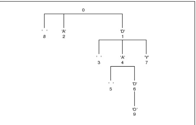
Huffman coding shares most characteristics of Shannon-Fano coding. It creates variable-length codes that are an integral number of bits. Symbols with higher probabilities get shorter codes. Huffman codes have the unique prefix attribute, which means they can be correctly decoded despite being variable length. Decoding a stream of Huffman codes is generally done by following a binary decoder tree.
Building the Huffman decoding tree is done using a completely different algorithm from that of the Shannon-Fano method. The Shannon-Fano tree is built from the top down, starting by assigning the most significant bits to each code and working down the tree until finished. Huffman codes are built from the bottom up, starting with the leaves of the tree and working progressively closer to the root.
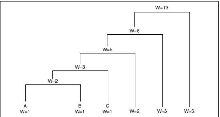
The procedure for building the tree is simple and elegant. The individual symbols are laid out as a string of leaf nodes that are going to be connected by a binary tree. Each node has a weight, which is simply the frequency or probability of the symbol’s appearance. The tree is then built with the following steps:
• The two free nodes with the lowest weights are located.
• A parent node for these two nodes is created. It is assigned a weight equal to the sum of the two child nodes.
• The parent node is added to the list of free nodes, and the two child nodes are removed from the list.
• One of the child nodes is designated as the path taken from the parent node when decoding a 0 bit. The other is arbitrarily set to the 1 bit.
• The previous steps are repeated until only one free node is left. This free node is designated the root of the tree.
This algorithm can be applied to the symbols used in the previous example. The five symbols in our message are laid out, along with their frequencies, as shown:
Symbol Count Info Cont. Info Bits SF Size SF Bits
A 15 1.38 20.68 2 30
B 7 2.48 17.35 2 14
C 6 2.70 16.20 2 12
D 6 2.70 16.20 3 18
E 5 2.96 14.82 3 15
These five nodes are going to end up as the leaves of the decoding tree. When the process first starts, they make up the entire list of free nodes.
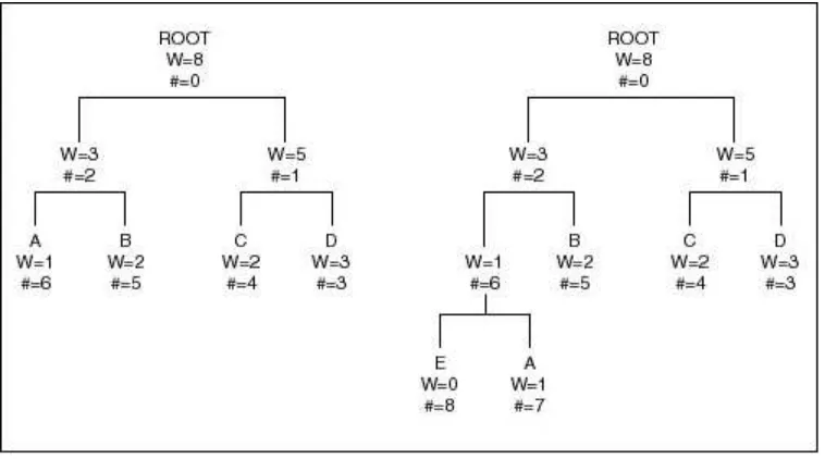
The first pass through the tree identifies the two free nodes with the lowest weights: D and E, with weights of 6 and 5. (The tie between C and D was broken arbitrarily. While the way that ties are broken affects the final value of the codes, it will not affect the compression ratio achieved.) These two nodes are joined to a parent node, which is assigned a weight of 11. Nodes D and E are then removed from the free list.
Once this step is complete, we know what the least significant bits in the codes for D and E are going to be. D is assigned to the 0 branch of the parent node, and E is assigned to the 1 branch. These two bits will be the LSBs of the resulting codes.
On the next pass through the list of free nodes, the B and C nodes are picked as the two with the lowest weight. These are then attached to a new parent node. The parent node is assigned a weight of 13, and B and C are removed from the free node list. At this point, the tree looks like that shown in Figure 3.2.
Figure 3.2 The Huffman tree after two passes.
On the next pass, the two nodes with the lowest weights are the parent nodes for the B/C and D/E pairs. These are tied together with a new parent node, which is assigned a weight of 24, and the children are removed from the free list. At this point, we have assigned two bits each to the Huffman codes for B, C, D, and E, and we have yet to assign a single bit to the code for A.
Finally, on the last pass, only two free nodes are left. The parent with a weight of 24 is tied with the A node to create a new parent with a weight of 39. After removing the two child nodes from the free list, we are left with just one parent, meaning the tree is complete. The final result looks like that shown in Figure 3.3.
Figure 3.3 The Huffman tree.
To determine the code for a given symbol, we have to walk from the leaf node to the root of the Huffman tree, accumulating new bits as we pass through each parent node. Unfortunately, the bits are returned to us in the reverse order that we want them, which means we have to push the bits onto a stack, then pop them off to generate the code. This strategy gives our message the code structure shown in the following table.
As you can see, the codes have the unique prefix property. Since no code is a prefix to another code, Huffman codes can be unambiguously decoded as they arrive in a stream. The symbol with the highest probability, A, has been assigned the fewest bits, and the symbol with the lowest probability, E, has been assigned the most bits.
Note, however, that the Huffman codes differ in length from Shannon-Fano codes. The code length for A is only a single bit, instead of two, and the B and C symbols have 3-bit codes instead of two bits. The following table shows what effect this has on the total number of bits produced by the message.
This adjustment in code size adds 13 bits to the number needed to encode the B and C symbols, but it saves 15 bits when coding the A symbol, for a net savings of 2 bits. Thus, for a message with an information content of 85.25 bits, Shannon-Fano coding requires 89 bits, but Huffman coding requires only 87.
In general, Shannon-Fano and Huffman coding are close in performance. But Huffman coding will always at least equal the efficiency of Shannon-Fano coding, so it has become the predominant coding method of its type. Since both algorithms take a similar amount of processing power, it seems sensible to take the one that gives slightly better performance. And Huffman was able to prove that this coding method cannot be improved on with any other integral bit-width coding stream.
Since D. A. Huffman first published his 1952 paper, “A Method for the Construction of Minimum Redundancy Codes,” his coding algorithm has been the subject of an overwhelming amount of additional research. Information theory journals to this day carry numerous papers on the
implementation of various esoteric flavors of Huffman codes, searching for ever better ways to use this coding method. Huffman coding is used in commercial compression programs, FAX machines, and even the JPEG algorithm. The next logical step in this book is to outline the C code needed to implement the Huffman coding scheme.
Huffman in C
A Huffman coding tree is built as a binary tree, from the leaf nodes up. Huffman may or may not have had digital computers in mind when he developed his code, but programmers use the tree data structure all the time.
A 0
B 100
C 101
D 110
E 111
Symbol Count
Shannon-Fano Size Shannon-Fano Bits Huffman Size Huffman Bits
A 15 2 30 1 15
B 7 2 14 3 21
C 6 2 12 3 18
D 6 3 18 3 18
Two programs used here illustrate Huffman coding. The compressor, HUFF-C, implements a simple order-0 model and a single Huffman tree to encode it. HUFF-E expands files compressed using HUFF-C. Both programs use a few pieces of utility code that will be seen throughout this book. Before we go on the actual Huffman code, here is a quick overview of what some of the utility modules do.
BITIO.C
Data-compression programs perform lots of input/output (I/O) that does reads or writes of
unconventional numbers of bits. Huffman coding, for example, reads and writes bits one at a time. LZW programs read and write codes that can range in size from 9 to 16 bits. The standard C I/O library defined in STDIO.H only accommodates I/O on even byte boundaries. Routines like putc() and getc() read and write single bytes, while fread() and fwrite() read and write whole blocks of bytes at a time. The library offers no help for programmers needing a routine to write a single bit at a time.
To support this conventional I/O in a conventional way, bit-oriented I/O routines are confined to a single source module, BITIO.C. Access to these routines is provided via a header file called BITIO.H, which contains a structure definition and several function prototypes.
Two routines open files for bit I/O, one for input and one for output. As defined in BITIO.H, they are
BIT_FILE *OpenInputBitFile( char *name ); BIT_FILE *OpenOutputBitFile ( char *name );
These two routines return a pointer to a new structure, BIT_FILE. BIT_FILE is also defined in BITIO.H as shown:
typedef struct bit_file { FILE *file;
unsigned char mask; int rack;
int pacifier_counter; } BIT_FILE:
OpenInputBitFile() or OpenOutputBitFile() perform a conventional fopen() call and store the returned FILE structure pointer in the BIT_FILE structure. The other two structure elements are initialized to their startup values, and a pointer to the resulting BIT_FILE structure is returned.
In BITIO.H, rack contains the current byte of data either read in from the file or waiting to be written out to the file. mask contains a single bit mask used either to set or clear the current output bit or to mask in the current input bit.
The two new structure elements, rack and mask, manage the bit-oriented aspect of a most significant bit in the I/O byte gets or returns the first bit, and the least significant bit in the I/O byte gets or returns the last bit. This means that the mask element of the structure is initialized to 0x80 when the BIT_FILE is first opened. During output, the first write to the BIT_FILE will set or clear that bit, then the mask element will shift to the next. Once the mask has shifted to the point at which all the bits in the output rack have been set or cleared, the rack is written out to the file, and a new rack byte is started.
rack have been returned, and the input routine can read in a new byte from the input file.
Two types of I/O routine