CRC Press Adaptive Digital Filters Signal Processing And Communications 2nd Edition Jul 2001 ISBN 0824705637 pdf

Adaptive Digital Filters

Second Edition, Revised and Expanded

Maurice G. Bellanger

Conservatoire National des Arts et Metiers (CNAM) Paris, France

M A R C E L

The first edition was published as Adaptive Digital Filters and Signal Analysis, Maurice G. Bellanger (Marcel Dekker, Inc., 1987).

ISBN: 0-8247-0563-7

This book is printed on acid-free paper.

Headquarters

Marcel Dekker, Inc.

270 Madison Avenue, New York, NY 10016 tel: 212-696-9000; fax: 212-685-4540

Eastern Hemisphere Distribution

Marcel Dekker AG

Hutgasse 4, Postfach 812, CH-4001 Basel, Switzerland tel: 41-61-261-8482; fax: 41-61-261-8896

World Wide Web http://www.dekker.com

The publisher offers discounts on this book when ordered in bulk quantities. For more information, write to Special Sales/Professional Marketing at the headquarters address above.

Copyright#2001 by Marcel Dekker, Inc. All Rights Reserved.

Neither this book nor any part may be reproduced or transmitted in any form or by any means, electronic or mechanical, including photocopying, microfilming, and recording, or by any information storage and retrieval system, without permission in writing from the publisher.

Current printing (last digit): 10 9 8 7 6 5 4 3 2 1

Signal Processing and Communications

Editorial Board

Maurice G. Ballanger,Conservatoire National des Arts et MÈtiers (CNAM), Paris Ezio Biglieri,Politecnico di Torino, Italy Sadaoki Furui,Tokyo Institute of Technology

Yih-Fang Huang,University of Notre Dame Nikhil Jayant,Georgia Tech University Aggelos K. Katsaggelos,Northwestern University

Mos Kaveh,University of Minnesota P. K. Raja Rajasekaran,Texas Instruments John Aasted Sorenson,IT University of Copenhagen

1. Digital Signal Processing for Multimedia Systems,edited by Keshab K. Parhi and Takao Nishitani

2. Multimedia Systems, Standards, and Networks, edited by Atul Puri and Tsuhan Chen

3. Embedded Multiprocessors: Scheduling and Synchronization, Sun-dararajan Sriram and Shuvra S. Bhattacharyya

4. Signal Processing for Intelligent Sensor Systems,David C. Swanson

5. Compressed Video over Networks,edited by Ming-Ting Sun and Amy R. Reibman

6. Modulated Coding for Intersymbol Interference Channels,Xiang-Gen Xia

7. Digital Speech Processing, Synthesis, and Recognition: Second Edi­ tion, Revised and Expanded,Sadaoki Furui

8. Modern Digital Halftoning,Daniel L. Lau and Gonzalo R. Arce

9. Blind Equalization and Identification,Zhi Ding and Ye (Geoffrey) Li

10. Video Coding for Wireless Communication Systems,King N. Ngan, Chi W. Yap, and Keng T. Tan

11. Adaptive Digital Filters: Second Edition, Revised and Expanded,

Maurice G. Bellanger

12. Design of Digital Video Coding Systems,Jie Chen, Ut-Va Koc, and K. J. Ray Liu

TM

13. Programmable Digital Signal Processors: Architecture, Program­ ming, and Applications,edited by Yu Hen Hu

14. Pattern Recognition and Image Preprocessing: Second Edition, Re­ vised and Expanded,Sing-Tze Bow

15. Signal Processing for Magnetic Resonance Imaging and Spectros­ copy,edited by Hong Yan

16. Satellite Communication Engineering,Michael O. Kolawole

Additional Volumes in Preparation

TM

Series Introduction

Over the past 50 years, digital signal processing has evolved as a major engineering discipline. The fields of signal processing have grown from the origin of fast Fourier transform and digital filter design to statistical spectral analysis and array processing, and image, audio, and multimedia processing, and shaped developments in high-performance VLSI signal processor design. Indeed, there are few fields that enjoy so many applications—signal processing is everywhere in our lives.

When one uses a cellular phone, the voice is compressed, coded, and modulated using signal processing techniques. As a cruise missile winds along hillsides searching for the target, the signal processor is busy proces-sing the images taken along the way. When we are watching a movie in HDTV, millions of audio and video data are being sent to our homes and received with unbelievable fidelity. When scientists compare DNA samples, fast pattern recognition techniques are being used. On and on, one can see the impact of signal processing in almost every engineering and scientific discipline.

Because of the immense importance of signal processing and the fast-growing demands of business and industry, this series on signal processing serves to report up-to-date developments and advances in the field. The topics of interest include but are not limited to the following:

. Signal theory and analysis . Statistical signal processing . Speech and audio processing . Image and video processing

. Multimedia signal processing and technology . Signal processing for communications

I hope this series will provide the interested audience with high-quality, state-of-the-art signal processing literature through research monographs, edited books, and rigorously written textbooks by experts in their fields.

Preface

The main idea behind this book, and the incentive for writing it, is that strong connections exist between adaptive filtering and signal analysis, to the extent that it is not realistic—at least from an engineering point of view—to separate them. In order to understand adaptive filters well enough to design them properly and apply them successfully, a certain amount of knowledge of the analysis of the signals involved is indispensable. Conversely, several major analysis techniques become really efficient and useful in products only when they are designed and implemented in an adaptive fashion. This book is dedicated to the intricate relationships between these two areas. Moreover, this approach can lead to new ideas and new techniques in either field.

The areas of adaptive filters and signal analysis use concepts from several different theories, among which are estimation, information, and circuit theories, in connection with sophisticated mathematical tools. As a conse-quence, they present a problem to the application-oriented reader. However, if these concepts and tools are introduced with adequate justification and illustration, and if their physical and practical meaning is emphasized, they become easier to understand, retain, and exploit. The work has therefore been made as complete and self-contained as possible, presuming a back-ground in discrete time signal processing and stochastic processes.

engineering. The gradient or least mean squares (LMS) adaptive filters are treated in Chapter 4. The theoretical aspects, engineering design options, finite word-length effects, and implementation structures are covered in turn. Chapter 5is entirely devoted to linear prediction theory and techni-ques, which are crucial in deriving and understanding fast algorithms opera-tions. Fast least squares (FLS) algorithms of the transversal type are derived and studied inChapter 6,with emphasis on design aspects and performance. Several complementary algorithms of the same family are presented in

Chapter 7to cope with various practical situations and signal types. Time and order recursions that lead to FLS lattice algorithms are pre-sented in Chapter 8,which ends with an introduction to the unified geo-metric approach for deriving all sorts of FLS algorithms. In other areas of signal processing, such as multirate filtering, it is known that rotations provide efficiency and robustness. The same applies to adaptive filtering, and rotation based algorithms are presented inChapter 9.The relationships with the normalized lattice algorithms are pointed out. The major spectral analysis and estimation techniques are described in Chapter 10, and the connections with adaptive methods are emphasized. Chapter 11 discusses circuits and architecture issues, and some illustrative applications, taken from different technical fields, are briefly presented, to show the significance and versatility of adaptive techniques. Finally,Chapter 12is devoted to the field of communications, which is a major application area.

At the end of several chapters, FORTRAN listings of computer subrou-tines are given to help the reader start practicing and evaluating the major techniques.

The book has been written with engineering in mind, so it should be most useful to practicing engineers and professional readers. However, it can also be used as a textbook and is suitable for use in a graduate course. It is worth pointing out that researchers should also be interested, as a number of new results and ideas have been included that may deserve further work.

I am indebted to many friends and colleagues from industry and research for contributions in various forms and I wish to thank them all for their help. For his direct contributions, special thanks are due to J. M. T. Romano, Professor at the University of Campinas in Brazil.

Contents

Series Introduction K. J. Ray Liu

Preface

1. Adaptive Filtering and Signal Analysis

2. Signals and Noise

3. Correlation Function and Matrix

4. Gradient Adaptive Filters

5. Linear Prediction Error Filters

6. Fast Least Squares Transversal Adaptive Filters

7. Other Adaptive Filter Algorithms

8. Lattice Algorithms and Geometrical Approach

9. Rotation-Based Algorithms

10. Spectral Analysis

11. Circuits and Miscellaneous Applications

1

Adaptive Filtering and Signal

Analysis

Digital techniques are characterized by flexibility and accuracy, two proper-ties which are best exploited in the rapidly growing technical field of adap-tive signal processing.

Among the processing operations, linear filtering is probably the most common and important. It is made adaptive if its parameters, the coeffi-cients, are varied according to a specified criterion as new information becomes available. That updating has to follow the evolution of the system environment as fast and accurately as possible, and, in general, it is asso-ciated with real-time operation. Applications can be found in any technical field as soon as data series and particularly time series are available; they are remarkably well developed in communications and control.

Conversely, adaptive techniques can be efficient instruments for perform-ing signal analysis. For example, an adaptive filter can be designed as an intelligent spectrum analyzer.

So, for all these reasons, it appears that learning adaptive filtering goes with learning signal analysis, and both topics are jointly treated in this book.

First, the signal analysis problem is stated in very general terms.

1.1.

SIGNAL ANALYSIS

By definition a signal carries information from a source to a receiver. In the real world, several signals, wanted or not, are transmitted and processed together, and the signal analysis problem may be stated as follows.

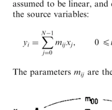
Let us consider a set of N sources which produce N variables

x0;x1;. . .;xN 1 and a set ofN corresponding receivers which give N

vari-ablesy0;y1;. . .;yN 1, as shown inFigure 1.1.The transmission medium is

assumed to be linear, and every receiver variable is a linear combination of the source variables:

yi¼

X

N 1

j¼0

mijxj; 0 4i4N 1 ð1:1Þ

The parametersmij are the transmission coefficients of the medium.

Now the problem is how to retrieve the source variables, assumed to carry the useful information looked for, from the receiver variables. It might also be necessary to find the transmission coefficients. Stated as such, the problem might look overly ambitious. It can be solved, at least in part, with some additional assumptions.

For clarity, conciseness, and thus simplicity, let us write equation (1.1) in matrix form:

Y_¼MX _ð1:2_Þ

with X_¼ x0 x1 .. .

x_N 1 2 6 6 6 4 3 7 7 7 5

; Y _¼

y0

y1 .. .

y_N 1 2 6 6 6 4 3 7 7 7 5 M_¼

m00 m01 m0N 1

m10 m11 m1N 1

.. .

.. .

mN 10 mN 1N 1

2 6 6 6 4 3 7 7 7 5

Now assume that thexi are random centered uncorrelated variables and

consider theNNmatrix

YYt_¼MXXtMt _ð1:3_Þ

whereMt denotes the transpose of the matrixM. Taking its mathematical expectation and noting that the transmission coefficients are deterministic variables, we get

E_½YYt_{Š ¼}ME_½XXt_ŠMt _ð1:4_Þ

Since the variablesxið0 4i4N 1Þare assumed to be uncorrelated, the

NN source matrix is diagonal:

E_½XXt_{Š ¼}

Px0 0 0

0 P_x1 0

.. . .. . . . . .. .

0 0 PxN 1

2 6 6 6 4 3 7 7 7 5¼

diag_½Px0;Px1;. . .;PxN 1Š

where

Pxi ¼E½x

2

is the power of the source with indexi. Thus, a decomposition of the receiver covariance matrix has been achieved:

E_½YYt_{Š ¼}Mdiag_½Px0;Px1;. . .;PxN 1ŠM

t

ð1:5_Þ

Finally, it appears possible to get the source powers and the transmission matrix from the diagonalization of the covariance matrix of the receiver variables. In practice, the mathematical expectation can be reached, under suitable assumptions, by repeated measurements, for example. It is worth noticing that if the transmission medium has no losses, the power of the sources is transferred to the receiver variables in totality, which corresponds to the relationMMt_¼IN; the transmission matrix is unitary in that case.

In practice, useful signals are always corrupted by unwanted externally generated signals, which are classified as noise. So, besides useful signal sources, noise sources have to be included in any real transmission system. Consequently, the number of sources can always be adjusted to equal the number of receivers. Indeed, for the analysis to be meaningful, the number of receivers must exceed the number of useful sources.

The technique presented above is used in various fields for source detec-tion and locadetec-tion (for example, radio communicadetec-tions or acoustics); the set of receivers is an array of antennas. However, the same approach can be applied as well to analyze a signal sequence when the data y_ðn_Þare linear combinations of a set of basic components. The problem is then to retrieve these components. It is particularly simple wheny_ðn_Þis periodic with period

N, because then the signal is just a sum of sinusoids with frequencies that are multiples of 1=N, and the matrix M in decomposition (1.5) is the discrete Fourier transform (DFT) matrix, the diagonal terms being the power spec-trum. For an arbitrary set of data, the decomposition corresponds to the representation of the signal as sinusoids with arbitrary frequencies in noise; it is a harmonic retrieval operation or a principal component analysis pro-cedure.

Rather than directly searching for the principal components of a signal to analyze it, extract its information, condense it, or clear it from spurious noise, we can approximate it by the output of a model, which is made as simple as possible and whose parameters are attributed to the signal. But to apply that approach, we need some characterization of the signal.

1.2.

CHARACTERIZATION AND MODELING

x_ðn_{Þ ¼}Ssin_ðn!_þ’_{Þ ð}1:6_Þ

whereSis the sinusoid amplitude,!is the angular frequency, and’is the phase. The same signal can also be represented and generated by the recur-rence relation

x_ðn_{Þ ¼ ð}2 cos!_Þx_ðn 1_Þ x_ðn 2_{Þ ð}1:7_Þ

forn50, and the initial conditions

x_ð 1_{Þ ¼}Ssin_ð !_þ’_Þ x_ð 2_{Þ ¼}Ssin_ð 2!_þ’_Þ

x_ðn_{Þ ¼}0 forn< 2

Recurrence relations play a key role in signal modeling as well as in adaptive filtering. The correspondence between time domain sequences and recur-rence relations is established by thez-transform, defined by

X_ðz_{Þ ¼} X

1

n¼ 1

x_ðn_Þz n _ð1:8_Þ

Waveform parameters are appropriate for synthetic signals, but for prac-tical signal analysis the correlation function r_ðp_Þ, in general, contains the relevant characteristics, as pointed out in the previous section:

r_ðp_{Þ ¼}E_½x_ðn_Þx_ðn p_{ފ ð}1:9_Þ

In the analysis process, the correlation function is first estimated and then used to derive the signal parameters of interest, the spectrum, or the recur-rence coefficients.

The recurrence relation is a convenient representation or modeling of a wide class of signals, which are those obtained through linear digital filtering of a random sequence. For example, the expression

x_ðn_{Þ ¼}e_ðn_Þ X

N

i¼1

aixðn iÞ ð1:10Þ

The coefficientsaiin (1.10) are the FIR, or transversal, linear prediction

coefficients of the signalx_ðn_Þ; they are actually the coefficients of the inverse FIR filter defined by

e_ðn_{Þ ¼}X

N

i¼0

aixðn iÞ; a0¼1 ð1:11Þ

The sequencee_ðn_Þis called the prediction error signal. The coefficients are designed to minimize the prediction error power, which, expressed as a matrix form equation is

E_½e2_ðn_{ފ ¼}AtE_½XXt_ŠA _ð1:12_Þ

So, for a given signal whose correlation function is known or can be estimated, the linear prediction (or AR modeling) problem can be stated as follows: find the coefficient vector A which minimizes the quantity

AtE_½XXt_ŠA subject to the constraint a0 ¼1. In that process, the power

of a white noise added to the useful input signal is magnified by the factor

AtA.

To provide a link between the direct analysis of the previous section and AR modeling, and to point out their major differences and similarities, we note that the harmonic retrieval, or principal component analysis, corre-sponds to the following problem: find the vector A which minimizes the valueAtE_½XXt_ŠAsubject to the constraintAtA_¼1. The frequencies of the sinusoids in the signal are then derived from the zeros of the filter with coefficient vectorA. For deterministic signals without noise, direct analysis and AR modeling lead to the same solution; they stay close to each other for high signal-to-noise ratios.

The linear prediction filter plays a key role in adaptive filtering because it is directly involved in the derivation and implementation of least squares (LS) algorithms, which in fact are based on real-time signal analysis by AR modeling.

1.3.

ADAPTIVE FILTERING

The optimization criterion

The algorithm for coefficient updating The programmable filter structure

The type of signals processed—mono- or multidimensional.

The optimization criterion is in general taken in the LS family in order to work with linear operations. However, in some cases, where simplicity of implementation and robustness are of major concern, the least absolute value (LAV) criterion can also be attractive; moreover, it is not restricted to minimum phase optimization.

The algorithms are highly dependent on the optimization criterion, and it is often the algorithm that governs the choice of the optimization criterion, rather than the other way round. In broad terms, the least mean squares (LMS) criterion is associated with the gradient algorithm, the LAV criterion corresponds to a sign algorithm, and the exact LS criterion is associated with a family of recursive algorithms, the most efficient of which are the fast least squares (FLS) algorithms.

The programmable filter can be a FIR or IIR type, and, in principle, it can have any structure: direct form, cascade form, lattice, ladder, or wave filter. Finite word-length effects and computational complexity vary with the structure, as with fixed coefficient filters. But the peculiar point with adaptive filters is that the structure reacts on the algorithm com-plexity. It turns out that the direct-form FIR, or transversal, structure is the simplest to study and implement, and therefore it is the most popular.

Multidimensional signals can use the same algorithms and structures as their monodimensional counterparts. However, computational complexity constraints and hardware limitations generally reduce the options to the simplest approaches.

The study of adaptive filtering begins with the derivation of the normal equations, which correspond to the LS criterion combined with the FIR direct form for the programmable filter.

1.4.

NORMAL EQUATIONS

In the following, we assume that real-time series, resulting, for example, from the sampling with periodT _¼1 of a continuous-time real signal, are processed.

Let H_ðn_Þ be the vector of the N coefficientshiðnÞof the programmable

filter at timen, and letX_ðn_Þbe the vector of theNmost recent input signal samples:

H_ðn_Þ

h0ðnÞ

h_Þ1ðn_Þ .. .

hN 1ðnÞ 2

6 6 6 4

3

7 7 7 5

; X_ðn_{Þ ¼}

x_ðn_Þ x_ðn 1_Þ

.. .

x_ðn_þ1 N_Þ

2

6 6 6 4

3

7 7 7

5 ð

1:13_Þ

The error signal"_ðn_Þis

"_ðn_{Þ ¼}y_ðn_Þ Ht_ðn_ÞX_ðn_{Þ ð}1:14_Þ

The optimization procedure consists of minimizing, at each time index, a cost functionJ_ðn_Þ, which, for the sake of generality, is taken as a weighted sum of squared error signal values, beginning after time zero:

J_ðn_{Þ ¼}X

n

p¼1

Wn p_½y_ðp_Þ Ht_ðn_ÞX_ðp_ފ2 _ð1:15_Þ

The weighting factor,W, is generally taken close to 1_ð0W 41). Now, the problem is to find the coefficient vectorH_ðn_Þwhich minimizes

J_ðn_Þ. The solution is obtained by setting to zero the derivatives ofJ_ðn_Þwith respect to the entrieshiðnÞof the coefficient vectorHðnÞ, which leads to

Xn

p¼1

Wn p_½y_ðp_Þ Ht_ðn_ÞX_ðp_ފX_ðp_{Þ ¼}0 _ð1:16_Þ

In concise form, (1.16) is

H_ðn_{Þ ¼}R_N1_ðn_Þr_yxðn_{Þ ð}1:17_Þ

with

RNðnÞ ¼

Xn

p¼1

ryxðnÞ ¼

Xn

p¼1

Wn pX_ðp_Þy_ðp_{Þ ð}1:19_Þ

If the signals are stationary, letR_xxbe theNNinput signal autocorrela-tion matrix and letr_yxbe the vector of cross-correlations between input and reference signals:

Rxx¼E½XðpÞXtðpފ; ryx¼E½XðpÞyðpފ ð1:20Þ

Now

E_½RNðnފ ¼

1 Wn

1 W Rxx; E½ryxðnފ ¼

1 Wn

1 W ryx ð1:21Þ

SoRNðnÞis an estimate of the input signal autocorrelation matrix, andryxðnÞ

is an estimate of the cross-correlation between input and reference signals. The optimal coefficient vectorHopt is reached whenngoes to infinity:

Hopt¼Rxx1ryx ð1:22Þ

Equations (1.22) and (1.17) are the normal (or Yule–Walker) equations for stationary and evolutive signals, respectively. In adaptive filters, they can be implemented recursively.

1.5.

RECURSIVE ALGORITHMS

The basic goal of recursive algorithms is to derive the coefficient vector

H_ðn_þ1_Þ from H_ðn_Þ. Both coefficient vectors satisfy (1.17). In these equa-tions, autocorrelation matrices and cross-correlation vectors satisfy the recursive relations

RNðnþ1Þ ¼WRNðnÞ þXðnþ1ÞXtðnþ1Þ ð1:23Þ

r_yxðn_þ1_{Þ ¼}Wr_yxðn_{Þ þ}X_ðn_þ1_Þy_ðn_þ1_{Þ ð}1:24_Þ

Now,

H_ðn_þ1_{Þ ¼}RN1ðnþ1Þ½WryxðnÞ þXðnþ1Þyðnþ1ފ

But

WryxðnÞ ¼ ½RNðnþ1Þ Xðnþ1ÞXtðnþ1ފHðnÞ

and

H_ðn_þ1_{Þ ¼}H_ðn_{Þ þ}RN1ðnþ1ÞXðnþ1Þ½yðnþ1Þ Xtðnþ1ÞHðnފ

which is the recursive relation for the coefficient updating. In that expres-sion, the sequence

e_ðn_þ1_{Þ ¼}y_ðn_þ1_Þ Xt_ðn_þ1_ÞH_ðn_{Þ ð}1:26_Þ

is called the a priori error signal because it is computed by using the coeffi-cient vector of the previous time index. In contrast, (1.14) defines the a posteriori error signal"_ðn_Þ, which leads to an alternative type of recurrence equation

H_ðn_þ1_{Þ ¼}H_ðn_{Þ þ}W 1R_N1_ðn_ÞX_ðn_þ1_Þe_ðn_þ1_{Þ ð}1:27_Þ

For large values of the filter orderN, the matrix manipulations in (1.25) or (1.27) lead to an often unacceptable hardware complexity. We obtain a drastic simplification by setting

RN1ðnþ1Þ IN

whereIN is theðNNÞunity matrix andis a positive constant called the

adaptation step size. The coefficients are then updated by

H_ðn_þ1_{Þ ¼}H_ðn_{Þ þ}X_ðn_þ1_Þe_ðn_þ1_{Þ ð}1:28_Þ

which leads to just doubling the computations with respect to the fixed-coefficient filter. The optimization process no longer follows the exact LS criterion, but LMS criterion. The productX_ðn_þ1_Þe_ðn_þ1_Þis proportional to the gradient of the square of the error signal with opposite sign, because differentiating equation (1.26) leads to

@e2_ðn_þ1_Þ

@hiðnÞ ¼

2x_ðn_þ1 i_Þe_ðn_þ1_Þ; 0 4i4N 1 _ð1:29_Þ

hence the name gradient algorithm.

The value of the step size has to be chosen small enough to ensure convergence; it controls the algorithm speed of adaptation and the residual error power after convergence. It is a trade-off based on the system engi-neering specifications.

can be avoided in the coefficient updating recursion by introducing the vector

G_ðn_{Þ ¼}RN1ðnÞXðnÞ ð1:30Þ

called the adaptation gain, which can be updated with the help of linear prediction filters. The corresponding algorithms are called FLS algorithms.

Up to now, time recursions have been considered, based on the cost function J_ðn_Þ defined by equation (1.15) for a set of N coefficients. It is also possible to work out order recursions which lead to the derivation of the coefficients of a filter of orderN_þ1 from the set of coefficients of a filter of order N. These order recursions rely on the introduction of a different set of filter parameters, called the partial correlation (PARCOR) coefficients, which correspond to the lattice structure for the programmable filter. Now, time and order recursions can be combined in various ways to produce a family of LS lattice adaptive filters. That approach has attractive advantages from the theoretical point of view— for example, signal orthogonalization, spectral whitening, and easy control of the minimum phase property—and also from the implementation point of view, because it is robust to word-length limitations and leads to flexible and modular realizations.

The recursive techniques can easily be extended to complex and multi-dimensional signals. Overall, the adaptive filtering techniques provide a wide range of means for fast and accurate processing and analysis of signals.

1.6.

IMPLEMENTATION AND APPLICATIONS

The circuitry designed for general digital signal processing can also be used for adaptive filtering and signal analysis implementation. However, a few specificities are worth point out. First, several arithmetic operations, such as divisions and square roots, become more frequent. Second, the processing speed, expressed in millions of instructions per second (MIPS) or in millions of arithmetic operations per second (MOPS), depending on whether the emphasis is on programming or number crunching, is often higher than average in the field of signal processing. Therefore specific efficient archi-tectures for real-time operation can be worth developing. They can be spe-cial multibus arrangements to facilitate pipelining in an integrated processor or powerful, modular, locally interconnected systolic arrays.

The block diagram of the configuration for system identification is shown in Figure 1.3. The input signalx_ðn_Þis fed to the system under analysis, which produces the reference signaly_ðn_Þ. The adaptive filter parameters and spe-cifications have to be chosen to lead to a sufficiently good model for the system under analysis. That kind of application occurs frequently in auto-matic control.

System correction is shown inFigure 1.4.The system output is the adap-tive filter input. An external reference signal is needed. If the reference signal

y_ðn_Þis also the system input signalu_ðn_Þ, then the adaptive filter is an inverse filter; a typical example of such a situation can be found in communications, with channel equalization for data transmission. In both application classes, the signals involved can be real or complex valued, mono- or multidimen-sional. Although the important case of linear prediction for signal analysis can fit into either of the aforementioned categories, it is often considered as an inverse filtering problem, with the following choice of signals:

y_ðn_{Þ ¼}0;u_ðn_{Þ ¼}e_ðn_Þ.

FIG. 1.3 Adaptive filter for system identification.

Another field of applications corresponds to the restoration of signals which have been degraded by addition of noise and convolution by a known or estimated filter. Adaptive procedures can achieve restoration by decon-volution.

The processing parameters vary with the class of application as well as with the technical fields. The computational complexity and the cost effi-ciency often have a major impact on final decisions, and they can lead to different options in control, communications, radar, underwater acoustics, biomedical systems, broadcasting, or the different areas of applied physics.

1.7.

FURTHER READING

The basic results, which are most necessary to read this book, in signal processing, mathematics, and statistics are recalled in the text as close as possible to the place where they are used for the first time, so the book is, to a large extent, self-sufficient. However, the background assumed is a work-ing knowledge of discrete-time signals and systems and, more specifically, random processes, discrete Fourier transform (DFT), and digital filter prin-ciples and structures. Some of these topics are treated in [1]. Textbooks which provide thorough treatment of the above-mentioned topics are [2– 4]. A theoretical veiw of signal analysis is given in [5], and spectral estima-tion techniques are described in [6]. Books on adaptive algorithms include [7–9]. Various applications of adaptive digital filters in the field of commu-nications are presented in [10–11].

REFERENCES

1. M. Bellanger,Digital Processing of Signals — Theory and Practice(3rd edn), John Wiley, Chichester, 1999.

2. A. V. Oppenheim, S. A. Willsky, and I. T. Young, Signals and Systems, Prentice-Hall, Englewood Cliffs, N.J., 1983.

3. S. K. Mitra and J. F. Kaiser, Handbook for Digital Signal Processing, John Wiley, New York, 1993.

4. G. Zeilniker and F. J. Taylor, Advanced Digital Signal Processing, Marcel Dekker, New York, 1994.

5. A. Papoulis,Signal Analysis, McGraw-Hill, New York, 1977.

6. L. Marple, Digital Spectrum Analysis with Applications, Prentice-Hall, Englewood Cliffs, N.J., 1987.

7. B. Widrow and S. D. Stearns, Adaptive Signal Processing, Prentice-Hall, Englewood Cliffs, N.J., 1985.

9. P. A. Regalia,Adaptive IIR Filtering in Signal Processing and Control, Marcel Dekker, New York, 1995.

10. C. F. N. Cowan and P. M. Grant,Adaptive Filters, Prentice-Hall, Englewood Cliffs, N.J., 1985.

2

Signals and Noise

Signals carry information from sources to receivers, and they take many different forms. In this chapter a classification is presented for the signals most commonly used in many technical fields.

A first distinction is between useful, or wanted, signals and spurious, or unwanted, signals, which are often called noise. In practice, noise sources are always present, so any actual signal contains noise, and a significant part of the processing operations is intended to remove it. However, useful sig-nals and noise have many features in common and can, to some extent, follow the same classification.

Only data sequences or time series are considered here, and the leading thread for the classification proposed is the set of recurrence relations, which can be established between consecutive data and which are the basis of several major analysis methods [1–3]. In the various categories, signals can be characterized by waveform functions, autocorrelation, and spectrum. An elementary, but fundamental, signal is introduced first—the damped sinusoid.

2.1.

THE DAMPED SINUSOID

Let us consider the following complex sequence, which is called the damped complex sinusoid, or damped cisoid:

y_ðn_{Þ ¼} eð

_þj!0Þn_{; n 50}

0; n<0

whereand!₀ are real scalars.

Thez-transform of that sequence is, by definition

Y_ðz_{Þ ¼}X

1

n¼0

y_ðn_Þz n _ð2:2_Þ

Hence

Y_ðz_{Þ ¼} 1

1 eð_þj!0Þ_z 1 ð2:3Þ

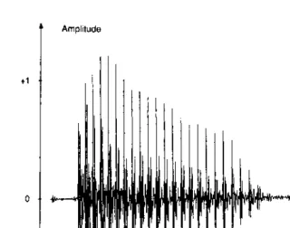
The two real corresponding sequences are shown inFigure 2.1(a).They are

y_ðn_{Þ ¼}yRðnÞ þjyIðnÞ ð2:4Þ

with

y_Rðn_{Þ ¼}encosn!₀; y_Iðn_{Þ ¼}ensinn!₀; n50 _ð2:5_Þ

Thez-transforms are

YRðzÞ ¼

1 _ðecos!0Þz 1

1 _ð2e_cos!

0Þz 1þe2z 2 ð

2:6_Þ

YIðzÞ ¼

1 _ðesin!_0Þz 1

1 _ð2e_cos!

0Þz 1þe2z 2 ð

2:7_Þ

In the complex plane, these functions have a pair of conjugate poles, which are shown inFigure 2.1(b)for <0 and_jjsmall. From (2.6) and (2.7) and also by direct inspection, it appears that the corresponding signals satisfy the recursion

yRðnÞ 2ecos!0yRðn 1Þ þ32yRðn 2Þ ¼0 ð2:8Þ

with initial values

yRð 1Þ ¼e cosð !0Þ; yRð 2Þ ¼e 2cosð 2!0Þ ð2:9Þ

and

yIð 1Þ ¼e sinð !0Þ; yIð 2Þ ¼e2sinð 2!0Þ ð2:10Þ

More generally, the one-sidedz-transform, as defined by (2.2), of equa-tion (2.8) is

YRðzÞ ¼

b1yRð 1Þ þb2½yRð 2Þ þyRð 1Þz 1Š

1_þb1z 1þb2z 2 ð

2:11_Þ

The above-mentioned initial values are then obtained by identifying (2.11) and (2.6), and (2.11) and (2.7), respectively.

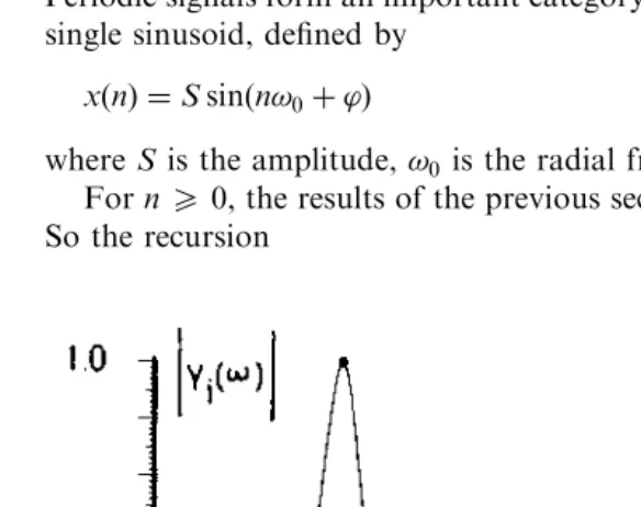
The energy spectra of the sequencesyRðnÞ andyÞIðnÞare obtained from

thez-transforms by replacingzbyej![4]. For example, the function_jY_Ið!_Þj

is shown in Figure 2.2; it is the frequency response of a purely recursive second-order filter section.

As n grows to infinity the signal y_ðn_Þ vanishes; it is nonstationary. Damped sinusoids can be used in signal analysis to approximate the spec-trum of a finite data sequence.

2.2.

PERIODIC SIGNALS

Periodic signals form an important category, and the simplest of them is the single sinusoid, defined by

x_ðn_{Þ ¼}Ssin_ðn!0þ’Þ ð2:12Þ

whereSis the amplitude,!0 is the radial frequency, and’is the phase.

Forn50, the results of the previous section can be applied with_¼0. So the recursion

x_ðn_Þ 2 cos!₀x_ðn 1_{Þ þ}x_ðn 2_{Þ ¼}0 _ð2:13_Þ

with initial conditions

x_ð 1_{Þ ¼}Ssin_ð !_0þ’_Þ; x_ð 2_{Þ ¼}Ssin_ð 2!_0þ’_{Þ ð}2:14_Þ

is satisfied. Thez-transform is

X_ðz_{Þ ¼}Ssin’ sinð !0þ’Þz

1

1 _ð2 cos!_0Þz 1_þz 2 ð2:15Þ

Now the poles are exactly on the unit circle, and we must consider the power spectrum. It cannot be directly derived from the z-transform. The sinusoid is generated for n>0 by the purely recursive second-order filter section inFigure 2.3with the above-mentioned initial conditions, the circuit input being zero. For a filter to cancel a sinusoid, it is necessary and suffi-cient to implement the inverse filter—that is, a filter which has a pair of zeros on the unit circle at the frequency of the sinusoid; such filters appear in linear prediction.

The autocorrelation function (ACF) of the sinusoid, which is a real sig-nal, is defined by

r_ðp_{Þ ¼} lim

N!1

1

N

X

N 1

n¼0

x_ðn_Þx_ðn p_{Þ ð}2:16_Þ

Hence,

r_ðp_{Þ ¼}S

2

2 cosp!0 Nlim!1

1 N S2 2 X N 1

n¼0

cos 2 2n p 2 !0þ’

ð2:17_Þ

and for any!0,

r_ðp_{Þ ¼}S

2

2 cosp!0 ð2:18Þ The power spectrum of the signal is the Fourier transform of the ACF; for the sinusoid it is a line with magnitudeS2=2 at frequency!₀.

Now, let us proceed to periodic signals. A periodic signal with periodN

consists of a sum of complex sinusoids, or cisoids, whose frequencies are integer multiples of 1=Nand whose complex amplitudesSkare given by the

discrete Fourier transform (DFT) of the signal data:

S0

S₁ .. .

SN 1 2 6 6 6 4 3 7 7 7 5¼ 1 N

1 1 1 1 W WN 1 .. . .. . . . . .. .

1 WN 1 WðN 1Þ2

2 6 6 6 4 3 7 7 7 5

x_ð0_Þ

x_ð1_Þ

.. .

x_ðN 1_Þ

2 6 6 6 4 3 7 7 7 5 ð

2:19_Þ

withW_¼e jð2=NÞ.

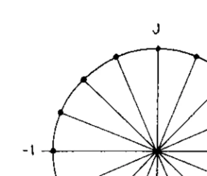
Following equation (2.3), with_¼0, we express the z-transform of the periodic signal by

X_ðz_{Þ ¼}X

N 1

k¼0

Sk

1 ejð2=NÞk_z 1 ð2:20Þ

and its poles are uniformly distributed on the unit circle as shown inFigure 2.4forNeven. Therefore, the signal x_ðn_Þsatisfies the recursion

XN

i¼0

aixðn iÞ ¼0 ð2:21Þ

where theai are the coefficients of the polynomialPðzÞ:

P_ðz_{Þ ¼}X

N

i¼0

a_iz 1 _¼Y

N

k¼1

ð1 ejð2=NÞkz 1_{Þ ð}2:22_Þ

Soa0¼1, and if all the cisoids are present in the periodic signal, thenaN¼

1 and a_i¼0 for 14i4N 1. The N complex amplitudes, or the real amplitudes and phases, are defined by the Ninitial conditions. If some of the N possible cisoids are missing, then the coefficients take on values according to the factors in the product (2.22).

r_ðp_{Þ ¼} 1 N

X

N 1

n¼0

x_ðn_Þxx_ðn p_{Þ ð}2:23_Þ

wherexx_ðn_Þis the complex conjugate ofx_ðn_Þ. According to the inverse DFT,

x_ðn_Þcan be expressed from its frequency components by

x_ðn_{Þ ¼}X

N 1

k¼0

Skejð2=NÞkn ð2:24Þ

Now, combining (2.24) and (2.23) gives

r_ðp_{Þ ¼}X

N 1

k¼0

jSkj2ejð2=NÞkp ð2:25Þ

and, forx_ðn_Þa real signal and for the configuration of poles shown inFigure 2.4withNeven,

r_ðp_{Þ ¼}S2_0þS_N2=2þ2 X

N=2 1

k¼1

jS_kj2cos 2

Nkp

ð2:26_Þ

The corresponding spectrum is made of lines at frequencies which are integer multiples of 1=N.

The same analysis as above can be carried out for a signal composed of a sum of sinusoids with arbitrary frequencies, which just implies that the

period N may grow to infinity. In that case, the roots of the polynomial

P_ðz_Þtake on arbitrary positions on the unit circle. Such a signal is said to be deterministic because it is completely determined by the recurrence relation-ship (2.21) and the set of initial conditions; in other words, a signal value at timen can be exactly calculated from the N preceding values; there is no innovation in the process; hence, it is also said to be predictable.

The importance of P_ðz_Þ is worth emphasizing, because it directly deter-mines the signal recurrence relation. Several methods of analysis primarily aim at finding out that polynomial for a start.

The above deterministic or predictable signals have discrete power spec-tra. To obtain continuous spectra, one must introduce random signals. They bring innovation in the processes.

2.3.

RANDOM SIGNALS

A random real signalx_ðn_Þis defined by a probability law for its amplitude at each timen. The law can be expressed as a probability densityp_ðx;n_Þdefined by

p_ðx;n_{Þ ¼} lim

x!0

Prob_½x4x_ðn_Þ4x_þx_Š

x ð2:27Þ

It is used to calculate, by ensemble averages, the statistics of the signal or process [5].

The signal is second order if it possesses a first-order momentm1ðnÞcalled

the mean value or expectation ofx_ðn_Þ, denoted E_½x_ðn_ފand defined by

m_1ðn_{Þ ¼}E_½x_ðn_{ފ ¼}

Z₁

1

xp_ðx;n_Þdx _ð2:28_Þ

and a second-order moment, called the covariance:

E_½x_ðn1Þxðn2ފ ¼m2ðn1;n2Þ ¼ Z ₁

1

Z₁

1

x1x2pðx1;x2;n1;n2Þdx1dx2 ð2:29Þ

wherep_ðx1;x2;;n1;n2Þis the joint probability density of the pair of random

variables_½x_ðn1Þ;xðn2ފ.

The signal isstationaryif its statistical properties are independent of the time indexn—that is, if the probability density is independent of timen:

p_ðx;n_{Þ ¼}p_ðx_{Þ ð}2:30_Þ

E_½x_ðn_{ފ ¼}

Z₁

1

xp_ðx_Þdx_¼m1 ð2:31Þ

E_½x_ðn_Þx_ðn p_{ފ ¼}r_ðp_{Þ ð}2:32_Þ

The functionr_ðp_Þis the (ACF) of the signal.

The statistical parameters are, in general, difficult to estimate or measure directly, because of the ensemble averages involved. A reasonably accurate measurement of an ensemble average requires that many process realiza-tions be available or that the experiment be repeated many times, which is often impractical. On the contrary, time averages are much easier to come by, for time series. Therefore the ergodicity property is of great practical importance; it states that, for a stationary signal, ensemble and time averages are equivalent:

m1¼E½xðnފ ¼ lim

N!1

1 2N_þ1

XN

n¼ N

x_ðn_{Þ ð}2:33_Þ

r_ðp_{Þ ¼}E_½x_ðn_Þx_ðn p_{ފ ¼} lim

N!1

1 2N_þ1

XN

n¼ N

x_ðn_Þx_ðn p_{Þ ð}2:34a_Þ

For complex signals, the ACF is

r_ðp_{Þ ¼}E_½x_ðn_Þxx_ðn p_{ފ ¼} lim

N!1

1 2N_þ1

XN

N

x_ðn_Þxx_ðn p_{Þ ð}2:34b_Þ

The factorx_ðn p_Þis replaced by its complex conjugatexx_ðn p_Þ; note that

r_ð0_Þis the signal power and is always a real number.

In the literature, the factor x_ðn_þp_Þ is generally taken to define r_ðp_Þ; however, we usex_ðn p_Þ throughout this book because it comes naturally in adaptive filtering.

In some circumstances, moments of orderk>2 might be needed. They are defined by

m_k¼

Z ₁

1

xkp_ðx_Þdx _ð2:35_Þ

and they can be calculated efficiently through the introduction of a function

F_ðu_Þ, called the characteristic function of the random variablexand defined by

F_ðu_{Þ ¼}

Z ₁

1

ejuxp_ðx_Þdx _ð2:36_Þ

F_ðu_{Þ ¼}X 1

k¼0

ðju_Þk

k! mk ð2:37Þ

SinceF_ðu_Þis the inverse Fourier transform of the probability densityp_ðx_Þ, it can be easy to calculate and can provide the high-order moments of the signal.

The moment of order 4 is used in the definition of the kurtosis Kx, or

coefficient of flatness of a probability distribution

K_x¼ E½x

4

ðn_ފ

E2_½x2_ðnފ ð2:38Þ

For example, a binary symmetric distribution (1 with equal probability) leads toKx¼1. For the Gaussian distribution of the next section,Kx¼3,

and for the exponential distribution

p_ðx_{Þ ¼} 1 pffiffiffi2e

ffiffi 2

p jxj=

ð2:39_Þ

K_x¼9.

An important concept is that of statistical independence of random vari-ables. Two random variables,x1andx2, are independent if and only if their

joint densityp_ðx1;x2Þis the product of the individual probability densities:

p_ðx1;x2Þ ¼pðx1Þpðx2Þ ð2:40Þ

which implies the same relationship for the characteristic functions:

F_ðu1;u2Þ ¼ Z Z1

1

ejðu1x1þu2x2Þ_pðx

1;x2Þdx1dx2 ð2:41Þ

and

F_ðu1;u2Þ ¼Fðu1ÞFðu2Þ ð2:42Þ

The correlation concept is related to linear dependency. Two noncorre-lated variables, such that E_½x1x2Š ¼0, have no linear dependency. But, in

general, that does not mean statistical independency, since higher-order dependency can exist.

2.4.

GAUSSIAN SIGNALS

A random variablex is said to be normally distributed or Gaussian if its probability law has a density p_ðx_Þ which follows the normal or Gaussian law:

p_ðx_{Þ ¼} 1

_xpffiffiffiffiffiffi2e

ðx mÞ2=22x _ð2:43Þ

The parameter m is the mean of the variable x; the variance _x2 is the second-order moment of the centered random variable _ðx m_Þ; _x is also called the standard deviation.

The characteristic function of the centered Gaussian variable is

F_ðu_{Þ ¼}e 2xu2=2

ð2:44_Þ

Now, using the series expansion (2.37), the moments are

m2kþ1¼0

m2¼x2; m4¼34x; m2k¼

2k!

2k_k!

2k

x ð2:45Þ

The normal law can be generalized to multidimensional random vari-ables. The characteristic function of a k-dimensional Gaussian variable

x_ðx1;x2;. . .;xkÞ is

F_ðu₁;u₂;. . .;u_{kÞ ¼}exp 1

2

Xk

i¼1 Xk

j¼1

r_iju_iu_j

!

ð2:46_Þ

withrij¼E½xixjŠ.

If the variables are not correlated, then they are independent, becauserij ¼0 fori_6¼j andF_ðu1;u2;. . .;ukÞis the product of the characteristic

func-tions. So noncorrelation means independence for Gaussian variables. A random signal x_ðn_Þ is said to be Gaussian if, for any set of k time values nið1 4i4kÞ, the k-dimensional random variablex¼ ½xðn1Þ;xðn2Þ;

. . .;x_ðnkފ is Gaussian. According to (2.46), the probability law of that

variable is completely defined by the ACFr_ðp_Þofx_ðn_Þ. The power spectral densityS_ðf_Þis obtained as the Fourier transform of the ACF:

S_ðf_{Þ ¼} X

1

p¼ 1

r_ðp_Þe j2pf _ð2:47_Þ

S_ðf_{Þ ¼}r_ð0_{Þ þ}2X

1

p¼1

r_ðp_Þcos_ð2pf_{Þ ð}2:48_Þ

If the data in the sequencex_ðn_Þare independent, thenr_ðp_Þreduces tor_ð0_Þand the spectrumS_ðf_Þis flat; the signal is then said to be white.

An important aspect of the Gaussian probability laws is that they pre-serve their character under any linear operation, such as convolution, filter-ing, differentiation, or integration.

Therefore, if a Gaussian signal is fed to a linear system, the output is also Gaussian. Moreover, there is a natural trend toward Gaussian probability densities, because of the so-called central limit theorem, which states that the random variable

x_¼ 1ffiffiffiffi

N

p X

N

i¼1

xi ð2:49Þ

where thexi areN independent identically distributed (i.i.d.) second-order

random variables, becomes Gaussian whenN grows to infinity.

The Gaussian approximation can reasonably be made as soon as N

exceeds a few units, and the importance of Gaussian densities becomes apparent because in nature many signal sources and, particularly, noise sources at the micro- or macroscopic levels add up to make the sequence to be processed. So Gaussian noise is present in virtually every signal pro-cessing application.

2.5.

SYNTHETIC, MOVING AVERAGE, AND

AUTOREGRESSIVE SIGNALS

In simulation, evaluation, transmission, test, and measurement, the data sequences used are often not natural but synthetic signals. They appear also in some analysis techniques, namely analysis by synthesis techniques.

Deterministic signals can be generated in a straightforward manner as isolated or recurring pulses or as sums of sinusoids. A diagram to produce a single sinusoid is shown inFigure 2.3.Note that the sinusoids in a sum must have different phases; otherwise an impulse shape waveform is obtained.

Flat spectrum signals are characterized by the fact that their energy is uniformly distributed over the entire frequency band. Therefore an approach to produce a deterministic white-noise-like waveform is to gener-ate a set of sinusoids uniformly distributed in frequency with the same amplitude but different phases.

rounding process. The magnitudes of these numbers are uniformly distrib-uted in the interval (0, 1), and the sequences obtained have a flat spectrum. Several probability densities can be derived from the uniform distribu-tion. Let the Gaussian, Rayleigh, and uniform densities bep_ðx_Þ,p_ðy_Þ, and

p_ðz_Þ, respectively. The Rayleigh density is

p_ðy_{Þ ¼} y

2exp

y2

22

" #

ð2:50_Þ

and the second-order moment of the corresponding random variable is 22, the mean ispffiffiffiffiffiffiffiffi=2, and the variance is_ð2 =2_Þ2. It is a density associated with the peak values of a narrowband Gaussian signal. The changes of variables

p_ðz_Þdz_¼dz_¼p_ðy_Þdy

leads to

dz

dy¼

y

2exp

y2

22

" #

Hence,

z_¼exp y

2

22

" #

and a Rayleigh sequencey_ðn_Þ is obtained from a uniform sequencez_ðn_Þ in the magnitude interval (0, 1) by the following operation:

y_ðn_{Þ ¼}pffiffiffiffiffiffiffiffiffiffiffiffiffiffiffiffiffiffiffiffiffiffiffi2 ln_½1=z_ðn_{ފ ð}2:51_Þ Now, independent Rayleigh and uniform sequences can be used to derive a Gaussian sequencex_ðn_Þ:

x_ðn_{Þ ¼}y_ðn_Þcos_½2z_ðn_{ފ ð}2:52_Þ

In the derivation, a companion variable is introduced:

x0_ðn_{Þ ¼}y_ðn_Þsin 2z_ðn_{Þ ð}2:53_Þ Now, let us consider the joint probability p_ðx;x0_Þ and apply the relation between rectangular and polar coordinates:

p_ðx;x0_Þdx dx0_¼p_ðx;x0_Þy dy dz_¼p_ðy_Þp_ðz_Þdy dz _ð2:54_Þ Then

p_ðx;x0_{Þ ¼} 1

2ypðyÞ ¼

1 22e

ðx2

þx02

Þ=22

and finally

p_ðx_{Þ ¼} 1 pffiffiffi2e

x2=22

ð2:56_Þ

The two variablesx_ðn_Þandx0_ðn_Þhave the same distribution and, considered jointly, they make a complex Gaussian noise of power 22. The above derivation shows that this complex noise can be represented in terms of its modulus, which has a Rayleigh distribution, and its phase, which has a uniform distribution.

Correlated random signals can be obtained by filtering a white sequence with either uniform or Gaussian amplitude probability density, as shown in

Figure 2.5.The filterH_ðz_Þcan take on different structures, corresponding to different models for the output signal [6].

The simplest type is the finite impulse response (FIR) filter, correspond-ing to the so-called movcorrespond-ing average (MA) model and defined by

H_ðz_{Þ ¼}X

N

i¼0

hiz i ð2:57Þ

and, in the time domain,

x_ðn_{Þ ¼}X

N

i¼0

hieðn iÞ ð2:58Þ

where thehi are the filter impulse response.

The output signal ACF is obtained by direct application of definition (2.34), considering that

E_½e2_ðn_{ފ ¼e}2; E_½e_ðn_Þe_ðn i_{ފ ¼}0 fori_6¼0

The result is

r_ðp_{Þ ¼} e2

P

N p

i¼0

h_ih_iþp; _jp_j 4N

0; _jp_j>N

8 <

: ð

2:59_Þ

Several remarks are necessary. First, the ACF has a finite length in accordance with the filter impulse response. Second, the output signal power_x2 is related to the input signal power by

2_x¼r_ð0_{Þ ¼e}2X

N

i¼0

h2i ð2:60Þ

Equation (2.60) is frequently used in subsequent sections. The power spectrum can be computed from the ACF r_ðp_Þ by using equation (2.48), but another approach is to useH_ðz_Þ, since it is available, via the equation

S_ðf_{Þ ¼}2_e X

N

i¼0

hiej2if

2

ð2:61_Þ

An infinite impulse response (IIR) filter corresponds to an autoregressive (AR) model. The equations are

H_ðz_{Þ ¼} 1

1 P

N

i¼1

aiz i

ð2:62_Þ

and, in the time domain,

x_ðn_{Þ ¼}e_ðn_{Þ þ}X

N

i¼1

aixðn iÞ ð2:63Þ

The ACF can be derived from the corresponding filter impulse response coefficientshi:

H_ðz_{Þ ¼}X

1

i¼0

hiz i ð2:64Þ

and, accordingly, it is an infinite sequence:

r_ðp_{Þ ¼}2e

X1

i¼0

hihiþp ð2:65Þ

The power spectrum is

S_ðf_{Þ ¼}

2

e

1 P

N

i¼1

aie j2if

2 ð2:66Þ

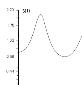
H_ðz_{Þ ¼} 1

ð1_þ0:80z 1_þ0:64z 2_{Þð1 1:23z} 1_þ0:64z 2_Þ

Since the spectrum of a real signal is symmetric about the zero frequency, only the band_½0;fs=2Š, wherefsis the sampling frequency, is represented.

For MA signals, the direct relation (2.59) has been derived between the ACF and filter coefficients. A direct relation can also be obtained here by multiplying both sides of the recursion definition (2.63) by x_ðn p_Þ and taking the expectation, which leads to

r_ð0_{Þ ¼}2_eþX

N

i¼1

airðiÞ ð2:67Þ

r_ðp_{Þ ¼}X

N

i¼1

airðp iÞ; p51 ð2:68Þ

Forp5N, the sequencer_ðp_Þis generated recursively from theNpreceding terms. For 04p4N 1, the above equations establish a linear depen-dence between the two sets of filter coefficients and the first ACF values.

They can be expressed in matrix form to derive the coefficients from the ACF terms:

r_ð0_Þ r_ð1_Þ r_ðN_Þ

r_ð1_Þ r_ð1_Þ r_ðN 1_Þ

.. . .. . . . . .. .

r_ðN_Þ r_ðN 1_Þ r_ð0_Þ

2 6 6 6 4 3 7 7 7 5 1 a₁ .. . aN 2 6 6 6 4 3 7 7 7 5¼ _e2 0 .. . 0 2 6 6 6 4 3 7 7 7 5 ð

2:69_Þ

Equation (2.69) is a normal equation, called the order N forward linear prediction equation, studied in a later chapter.

To complete the AR signal analysis, note that the generating filter impulse response is

hp¼rðpÞ

XN

i¼1

airðpþiÞ ð2:70Þ

This equation is a direct consequence of definition relations (2.63) and (2.64), if we notice that

hp¼E½xðnÞeðn pފ ð2:71Þ

Since r_ðp_{Þ ¼}r_ð p_Þ, equation (2.68) shows that the impulse response hp is

zero for negativep, which reflects the filter causality.

It is also possible to relate the AC function of an AR signal to the poles of the generating filter.

For complex poles, the filter z-transfer function can be expressed in factorized form:

H_ðz_{Þ ¼} 1

Q

N=2

i¼1ð

1 Piz 1Þð1 PPiz 1Þ

ð2:72_Þ

Using the equality

S_ðf_{Þ ¼}2ejHðzÞHðz 1Þjjzj¼1¼ X1

p¼ 1 r_ðp_Þz p

jzj¼1

ð2:73_Þ

the series development of the productH_ðz_ÞH_ðz 1_Þleads to the AC function of the AR signal. The rational function decomposition ofH_ðz_ÞH_ðz 1_Þyields, after simplification,

r_ðp_{Þ ¼}X

N=q

i¼1

_ijPijncos½nArgðpiÞ þiŠ ð2:74Þ

where the real parametersiandiare the parameters of the decomposition

It is worth pointing out that the same expression is obtained for the generating filter of the type FIR/IIR, but then the parameters _i and _i

are no longer related to the poles: they are independent.

A limitation of AR spectra is that they do not take on zero values, whereas MA spectra do. So it may be useful to combine both [7].

2.6.

ARMA SIGNALS

An ARMA signal is obtained through a filter with a rational z-transfer function:

H_ðz_{Þ ¼}

PN

i¼0

b_iz 1

1 P

N

i¼1

aiz 1

ð2:75_Þ

In the time domain,

x_ðn_{Þ ¼}X

N

i¼0

bieðn iÞ þ

XN

i¼1

aixðn iÞ ð2:76Þ

The denominator and numerator polynomials of H_ðz_Þ can always be assumed to have the same order; if necessary, zero coefficients can be added.

The power spectral density is

S_ðf_{Þ ¼}2e

PN

i¼0

bie j2if

2

1 P

N

i¼1

aie j2if

2 ð2:77Þ

A direct relation between the ACF and the coefficients is obtained by multiplying both sides of the time recursion (2.76) byx_ðn p_Þand taking the expectation:

r_ðp_{Þ ¼}X

N

i¼1

a_ir_ðp i_{Þ þ}X

N

i¼0

b_iE_ðe_ðn i_Þx_ðn p_{ފ ð}2:78_Þ

r_ðN_Þ r_ðN 1_Þ r_ð0_Þ

r_ðN_þ1_Þ r_ðN_Þ r_ð1_Þ

.. . .. . . . . .. .

r_ð2N_Þ r_ð2N 1_Þ r_ðN_Þ

2 6 6 6 4 3 7 7 7 5 1 a₁ .. . aN 2 6 6 6 4 3 7 7 7 5¼

b0bN

_e2 0 .. . 0 2 6 6 6 4 3 7 7 7 5 ð

2:79_Þ

For p>N, the sequence r_ðp_Þ is again generated recursively from the N

preceding terms.

The relationship between the first_ðN_þ1_ÞACF terms and the filter coef-ficients can be established through the filter impulse response, whose coeffi-cientshi satisfy, by definition,

x_ðn_{Þ ¼}X 1

i¼0

hieðn iÞ ð2:80Þ

Now replacingx_ðn i_Þin (2.76) gives

x_ðn_{Þ ¼}X

N

i¼0

bieðn iÞ þ

XN

i¼1

ai

X1

j¼0

hjeðn i jÞ

and

x_ðn_{Þ ¼}X

N

i¼0

b_ie_ðn i_{Þ þ}X 1

k¼1

e_ðn k_ÞX

N

i¼1

a_ih_{k i ð}2:81_Þ

Clearly, the impulse response coefficients can be computed recursively:

h0¼b0; hk¼0 fork<0

hk¼bkþ

XN

i¼1

aihk i; k51

ð2:82_Þ

In matrix form, for theN_þ1 first terms we have 1 0 0 0

a1 1 0 0

a2 a1 1 0

.. . .. . .. . . . . .. .

aN aN 1 aN 2 1

2 6 6 6 6 6 4 3 7 7 7 7 7 5

h0 0 0 0

h1 h0 0 0

h2 h1 h0 0

.. . .. . .. . . . . .. .

hN hN 1 hN 2 h0

2 6 6 6 6 6 4 3 7 7 7 7 7 5 ¼

b0 0 0 0

b1 b0 0 0

b2 b1 b0 0

.. . .. . .. . . . . .. .

b_N b_{N 1} b_{N 2} b₀

2 6 6 6 6 6 4 3 7 7 7 7 7 5

Coming back to the ACF and (2.78), we have

XN

i¼0

biE½eðn iÞxðn pފ ¼e2

XN

i¼0

bihi p

and, after simple manipulations,

r_ðp_{Þ ¼}X

N

i¼1

a_ir_ðp i_{Þ þe}2X

N p

j¼0

b_jþph_{j ð}2:84_Þ

Now, introducing the variable

d_ðp_{Þ ¼}X

N p

j¼0

bjþphj ð2:85Þ

we obtain the matrix equation

A r_ð0_Þ

r_ð1_Þ

.. .

r_ðN_Þ

2 6 6 6 4 3 7 7 7 5þ A0

r_ð0_Þ

r_ð 1_Þ

.. .

r_ð N_Þ

2 6 6 6 4 3 7 7 7 5¼ 2e

d_ð0_Þ

d_ð1_Þ

.. .

d_ðN_Þ

2 6 6 6 4 3 7 7 7 5 ð

2:86_Þ

where

A_¼

1 0 0

a1 1 0

.. . .. . . . . .. .

aN aN 1 1

2 6 6 6 4 3 7 7 7 5

A0_¼

0 a₁ a_N

0 a2 0 .. . .. . .. .

0 aN

0 0 0

2 6 6 6 6 6 4 3 7 7 7 7 7 5

For real signals, the first_ðN_þ1_ÞACF terms are obtained from the equation

r_ð0_Þ

r_ð1_Þ

.. .

r_ðN_Þ

2 6 6 6 4 3 7 7 7 5¼

_e2_½A_þ A0_Š 1 d_ð0_Þ

d_ð1_Þ

.. .

d_ðN_Þ

2 6 6 6 4 3 7 7 7 5 ð

2:87_Þ

In summary, the procedure to calculate the ACF of an ARMA signal from the generating filter coefficients is as follows:

. .

.

. .

.

. .

.

. .

1. Compute the first _ðN_þ1_Þterms of the filter impulse response through recursion (2.82).

2. Compute the auxiliary variablesd_ðp_Þfor 0 4p4N.

3. Compute the first_ðN_þ1_ÞACF terms from matrix equation (2.87). 4. Use recursion (2.68) to deriver_ðp_Þwhenp5N_þ1.

Obviously, finding the ACF is not a simple task, particularly for large filter orders N. Conversely, the filter coefficients and input noise power can be retrieved from the ACF. First the AR coefficientsai and the scalar

b0bNe2 can be obtained from matrix equation (2.79). Next, from the time

domain definition (2.76), the following auxiliary signal can be introduced:

u_ðn_{Þ ¼}x_ðn_Þ X

N

i¼1

a_ix_ðn i_{Þ ¼}e_ðn_{Þ þ}X

N

i¼1

b_ie_ðn i_{Þ ð}2:88_Þ

whereb0¼1 is assumed.

The ACFruðpÞof the auxiliary signaluðnÞis derived from the ACF ofxðnÞ

by the equation

ruðpÞ ¼E½uðnÞuðn pފ

¼r_ðp_Þ X

N

i¼1

airðpþiÞ

XN

i¼1

airðp iÞ þ

XN

i¼1 XN

j¼1

aiajrðpþj iÞ

or, more concisely by

ruðpÞ ¼

XN

i¼ N

cirðp iÞ ð2:89Þ

where

ci¼c i; c0¼1þ XN

j¼1

a2j

c_i¼ a_iþ X

N

j¼iþ1

a_ja_{j i}

ð2:90_Þ

ButruðpÞcan also be expressed in terms of MA coefficients, because of the

second equation in (2.88). The corresponding expressions, already given in the previous section, are

ruðpÞ ¼

2

e

P

N p

i¼0

bibiþp; jpj 4N

0; _jp_j>N

8 <

From these N_þ1 equations, the input noise power 2_e and the MA coefficients bið1 4i4N;b0¼1Þ can be derived from iterative Newton–

Raphson algorithms. It can be verified that b0bNe2 equals the value we

previously found when solving matrix equation (2.79) for AR coefficients. The spectral densityS_ðf_Þcan be computed with the help of the auxiliary signalu_ðn_Þby considering the filtering operation

x_ðn_{Þ ¼}u_ðn_{Þ þ}X

N

i¼1

aixðn iÞ ð2:91Þ

which, in the spectral domain, corresponds to

S_ðf_{Þ ¼}

ruð0Þ þ2

PN

p¼1

ruðpÞcosð2pfÞ

1 P

N

i¼1

aie j2if

2 ð2:92Þ

This expression is useful in spectral analysis.

Until now, only real signals have been considered in this section. Similar results can be obtained with complex signals by making appropriate com-plex conjugations in equations. An important difference is that the ACF is no longer symmetrical, which can complicate some