Computability and Complexity Theory pdf pdf

Editors

David Gries

Fred B. Schneider

For further volumes:

Computability and

Complexity Theory

Second Edition

Computer Science Department Boston University

Boston Massachusetts USA

homer@bu.edu

Series Editors

David Gries

Department of Computer Science Upson Hall

Cornell University

Ithaca, NY 14853-7501, USA

Department of Computer Science and Engineering

University at Buffalo

The State University of New York Buffalo New York

USA

selman@buffalo.edu

Fred B. Schneider

Department of Computer Science Upson Hall

Cornell University

Ithaca, NY 14853-7501, USA

ISSN 1868-0941 e-ISSN 1868-095X ISBN 978-1-4614-0681-5 e-ISBN 978-1-4614-0682-2 DOI 10.1007/978-1-4614-0682-2

Springer New York Dordrecht Heidelberg London

Library of Congress Control Number: 2011941200 © Springer Science+Business Media, LLC 2011

All rights reserved. This work may not be translated or copied in whole or in part without the written permission of the publisher (Springer Science+Business Media, LLC, 233 Spring Street, New York, NY 10013, USA), except for brief excerpts in connection with reviews or scholarly analysis. Use in connection with any form of information storage and retrieval, electronic adaptation, computer software, or by similar or dissimilar methodology now known or hereafter developed is forbidden.

The use in this publication of trade names, trademarks, service marks, and similar terms, even if they are not identified as such, is not to be taken as an expression of opinion as to whether or not they are subject to proprietary rights.

Printed on acid-free paper

The theory of computing provides computer science with concepts, models, and formalisms for reasoning about both the resources needed to carry out computations and the efficiency of the computations that use these resources. It provides tools to measure the difficulty of combinatorial problems both absolutely and in comparison with other problems. Courses in this subject help students gain analytic skills and enable them to recognize the limits of computation. For these reasons, a course in the theory of computing is usually required in the graduate computer science curriculum.

The harder question to address is which topics such a course should cover. We believe that students should learn the fundamental models of computation, the limitations of computation, and the distinctions between feasible and intractable. In particular, the phenomena of NP-completeness and NP-hardness have pervaded much of science and transformed computer science. One option is to survey a large number of theoretical subjects, typically focusing on automata and formal languages. However, these subjects are less important to theoretical computer science, and to computer science as a whole, now than in the past. Many students have taken such a course as part of their undergraduate education. We chose not to take that route because computability and complexity theory are the subjects that we feel deeply about and that we believe are important for students to learn. Furthermore, a graduate course should be scholarly. It is better to treat important topics thoroughly than to survey the field.

This textbook is intended for use in an introductory graduate course in theoretical computer science. It contains material that should be core knowledge in the theory of computation for all graduate students in computer science. It is self-contained and is best suited for a one-semester course. Most of the text can be covered in one semester by moving expeditiously through the core material of Chaps.1through5

and then covering parts of Chap.6. We will give more details about this below. As a graduate course, students should have some prerequisite preparation. The ideal preparation would be the kind of course that we mentioned above: an undergraduate course that introduced topics such as automata theory, formal languages, computability theory, or complexity theory. We stress, however, that

there is nothing in such a course that a student needs to know before studying this text. Our personal experience suggests that we cannot presume that all of our students have taken such an undergraduate course. For those students who have not, we advise that they need at least some prior exposure that will have developed mathematical skills. Prior courses in mathematical logic, algebra (at the level of groups, rings, or fields), or number theory, for example, would all serve this purpose. Despite the diverse backgrounds of our students, we have found that graduate students are capable of learning sophisticated material when it is explained clearly and precisely. That has been our goal in writing this book.

This book also is suitable for advanced undergraduate students who have satisfied the prerequisites. It is an appropriate first course in complexity theory for students who will continue to study and work in this subject area.

The text begins with a preliminary chapter that gives a brief description of several topics in mathematics. We included this in order to keep the book self-contained and to ensure that all students have a common notation. Some of these sections simply enable students to understand some of the important examples that arise later. For example, we include a section on number theory and algebra that includes all that is necessary for students to understand that primality belongs to NP.

The text starts properly with classical computability theory. We build complexity theory on top of that. Doing so has the pedagogical advantage that students learn a qualitative subject before advancing to a quantitative one. Also, the concepts build from one to the other. For example, although we give a complete proof that the satisfiability problem is NP-complete, it is easy for students to understand that the bounded halting problem is NP-complete, because they already know that the classical halting problem is c.e.-complete.

We use the termspartial computableandcomputably enumerable (c.e.)instead of the traditional terminology,partial recursiveandrecursively enumerable (r.e.), respectively. We do so simply to eliminate confusion. Students of computer science know of “recursion” as a programming paradigm. We do not prove here that Turing-computable partial functions are equivalent to partial recursive functions, so by not using that notation, we avoid the matter altogether. Although the notation we are using has been commonplace in the computability theory and mathematical logic community for several years, instructors might want to advise their students that the older terminology seems commonplace within the theoretical computer science community. Computable functions are defined on the set of words over a finite alphabet, which we identify with the set of natural numbers in a straightforward manner. We use the termeffective, in the nontechnical, intuitive sense, to denote computational processes on other data types. For example, we will say that a set of Turing machines is “effectively enumerable” if its set of indices is computably enumerable.

it is possible to begin the study of complexity theory after learning the first five sections of Chap.4and at least part of Sect.3.9on oracle Turing machines, Turing reductions, and the arithmetical hierarchy.

In Chap.5, we treat general properties of complexity classes and relationships between complexity classes. These include important older results such as the space and time hierarchy theorems, as well as the more recent result of Immerman and Szelepcs´enyi that space-bounded classes are closed under complements. Instructors might be anxious to get to NP-complete problems (Chap.6) and NP-hard problems (Chap.7), but students need to learn the basic results of complexity theory and it is instructive for them to understand the relationships between P, NP, and other deterministic and nondeterministic, low-level complexity classes. Students should learn that nondeterminism is not well understood in general, that P =? NP is not an isolated question, and that other classes have complete problems as well (which we take up in Chap.7). Nevertheless, Chap.5is a long chapter. Many of the results in this chapter are proved by complicated Turing-machine simulations and counting arguments, which give students great insight, but can be time-consuming to cover. For this reason, instructors might be advised to survey some of this material if the alternative would mean not having sufficient time for the later chapters.

At long last we have written this second part, and here it is. We corrected a myriad of typos, a few technical glitches, and some pedagogical issues in the first part.

Chapter 8, the first of the new chapters, is on nonuniformity. Here we study Boolean circuits, advice classes, define P/poly, and establish the important result of Karp–Lipton. Then we define and show basic properties of Sch¨oning’s low and high hierarchies. We need this for results that will come later in Chap.10. Specifically, in that chapter we prove that the Graph Nonisomorphism Problem (GNI) is in the operator class BP_·NP and that the Graph Isomorphism Problem (GI) is in the low hierarchy. Then it follows immediately that GI cannot be NP-complete unless the polynomial hierarchy collapses. Of course, primarily this chapter studies properties of the fundamental probabilistic complexity classes.

We study the alternating Turing machine and uniform circuit classes, especially NC, in Chap.9. In the next chapter, we introduce counting classes and prove the famous results of Valiant and Vazirani and of Toda. The text ends with a thorough treatment of the proof that IP is identical to PSPACE, including worked-out examples. We include a section on Arthur-Merlin games and point worked-out that BP_·NP=AM, thereby establishing some of the results that classify this class.

We have found that the full text can be taught in one academic year. We hope that the expanded list of topics gives instructors flexibility in choosing topics to cover.

Thanks to everyone who sent us comments and corrections, and a special thanks to our students who demonstrated solvability of critical homework exercises.

Boston and Buffalo Steven Homer

Alan Selman

1 Preliminaries. . . 1

1.1 Words and Languages.. . . 1

1.2 K-adic Representation.. . . 2

1.3 Partial Functions. . . 3

1.4 Graphs. . . 4

1.5 Propositional Logic. . . 5

1.5.1 Boolean Functions. . . 7

1.6 Cardinality.. . . 8

1.6.1 Ordered Sets . . . 10

1.7 Elementary Algebra. . . 10

1.7.1 Rings and Fields. . . 10

1.7.2 Groups.. . . 15

1.7.3 Number Theory.. . . 17

2 Introduction to Computability. . . 23

2.1 Turing Machines . . . 24

2.2 Turing Machine Concepts. . . 26

2.3 Variations of Turing Machines.. . . 28

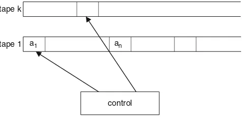
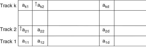
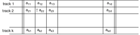
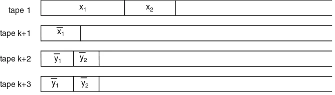
2.3.1 Multitape Turing Machines. . . 29

2.3.2 Nondeterministic Turing Machines. . . 32

2.4 Church’s Thesis. . . 35

2.5 RAMs. . . 36

2.5.1 Turing Machines for RAMS . . . 40

3 Undecidability. . . 41

3.1 Decision Problems. . . 41

3.2 Undecidable Problems. . . 42

3.3 Pairing Functions.. . . 45

3.4 Computably Enumerable Sets. . . 47

3.5 Halting Problem, Reductions, and Complete Sets. . . 50

3.5.1 Complete Problems. . . 52

3.6 S-m-nTheorem. . . 53

3.7 Recursion Theorem. . . 56

3.8 Rice’s Theorem.. . . 58

3.9 Turing Reductions and Oracle Turing Machines. . . 60

3.10 Recursion Theorem: Continued. . . 67

3.11 References. . . 71

3.12 Additional Homework Problems. . . 71

4 Introduction to Complexity Theory. . . 75

4.1 Complexity Classes and Complexity Measures. . . 76

4.1.1 Computing Functions. . . 79

4.2 Prerequisites. . . 79

5 Basic Results of Complexity Theory. . . 81

5.1 Linear Compression and Speedup.. . . 82

5.2 Constructible Functions. . . 89

5.2.1 Simultaneous Simulation.. . . 90

5.3 Tape Reduction.. . . 93

5.4 Inclusion Relationships. . . 99

5.4.1 Relations Between the Standard Classes. . . 107

5.5 Separation Results. . . 109

5.6 Translation Techniques and Padding. . . 113

5.6.1 Tally Languages. . . 116

5.7 Relations Between the Standard Classes: Continued.. . . 117

5.7.1 Complements of Complexity Classes: The Immerman–Szelepcs´enyi Theorem. . . 118

5.8 Additional Homework Problems. . . 122

6 Nondeterminism and NP-Completeness. . . 123

6.1 Characterizing NP. . . 124

6.2 The Class P. . . 125

6.3 Enumerations. . . 127

6.4 NP-Completeness. . . 129

6.5 The Cook–Levin Theorem.. . . 131

6.6 More NP-Complete Problems. . . 136

6.6.1 The Diagonal Set Is NP-Complete. . . 137

6.6.2 Some Natural NP-Complete Problems. . . 138

6.7 Additional Homework Problems. . . 142

7 Relative Computability. . . 145

7.1 NP-Hardness. . . 147

7.2 Search Problems.. . . 150

7.3 The Structure of NP. . . 153

7.3.1 Composite Number and Graph Isomorphism. . . 157

7.3.2 Reflection. . . 160

7.4 The Polynomial Hierarchy.. . . 161

7.5 Complete Problems for Other Complexity Classes. . . 169

7.5.2 Exponential Time. . . 173

7.5.3 Polynomial Time and Logarithmic Space. . . 174

7.5.4 A Note on Provably Intractable Problems. . . 178

7.6 Additional Homework Problems. . . 178

8 Nonuniform Complexity. . . 181

8.1 Polynomial Size Families of Circuits . . . 184

8.1.1 An Encoding of Circuits. . . 187

8.1.2 Advice Classes. . . 188

8.2 The Low and High Hierarchies. . . 191

9 Parallelism. . . 201

9.1 Alternating Turing Machines. . . 201

9.2 Uniform Families of Circuits. . . 209

9.3 Highly Parallelizable Problems. . . 213

9.4 Uniformity Conditions. . . 216

9.5 Alternating Turing Machines and Uniform Families of Circuits. . . 219

10 Probabilistic Complexity Classes. . . 225

10.1 The Class PP. . . 225

10.2 The Class RP. . . 229

10.2.1 The Class ZPP. . . 230

10.3 The Class BPP. . . 231

10.4 Randomly Chosen Hash Functions. . . 237

10.4.1 Operators.. . . 239

10.5 The Graph Isomorphism Problem. . . 242

10.6 Additional Homework Problems. . . 246

11 Introduction to Counting Classes. . . 247

11.1 Unique Satisfiability . . . 249

11.2 Toda’s Theorem. . . 253

11.2.1 Results on BPP and⊕P. . . 253

11.2.2 The First Part of Toda’s Theorem.. . . 257

11.2.3 The Second Part of Toda’s Theorem.. . . 257

11.3 Additional Homework Problems. . . 260

12 Interactive Proof Systems. . . 261

12.1 The Formal Model. . . 261

12.2 The Graph Non-Isomorphism Problem. . . 263

12.3 Arthur-Merlin Games. . . 265

12.4 IP Is Included in PSPACE . . . 267

12.5 PSPACE Is Included in IP . . . 270

12.5.1 The Language ESAT . . . 270

12.5.2 True Quantified Boolean Formulas. . . 274

12.5.3 The Proof.. . . 275

References. . . 283

Author Index. . . 289

Preliminaries

We begin with a limited number of mathematical notions that a student should know before beginning with this text. This chapter is short because we assume some earlier study of data structures and discrete mathematics.

1.1

Words and Languages

In the next chapter we will become familiar with models of computing. The basic data type of our computers will be “symbols,” for our computers manipulate symbols. The notion of symbol is undefined, but we define several more concepts in terms of symbols.

A finite setΣ ={a1, . . . ,ak} of symbols is called a finite alphabet. A wordis

a finite sequence of symbols. Thelengthof a wordw, denoted_|w_|, is the number of symbols composing it. The emptyword is the unique word of length 0 and is denoted asλ. Note thatλ isnota symbol in the alphabet. The empty word is not a set, so do not confuse the empty wordλ with the empty set /0.

Σ∗_{denotes the set of all words over the alphabetΣ. Alanguageis a set of words.}

That is,Lis a language if and only ifL_⊆Σ∗_{. Aprefixof a word is a substring that}

begins the word.

Example 1.1. Letw=abcce. The prefixes ofware λ,a,ab,abc,abcc,abcce.

Definesuffixessimilarly.

Theconcatenationof two wordsxandyis the wordxy. For any wordw,λw= wλ=w. Ifx=uvw, thenvis a subword ofx. Ifuandware not bothλ, thenvis a proper subword.

S. Homer and A.L. Selman,Computability and Complexity Theory, Texts in Computer Science, DOI 10.1007/978-1-4614-0682-2 1, © Springer Science+Business Media, LLC 2011

Some operations on languages:

union L1∪L2

intersection L1∩L2

complement L=Σ∗_−L

concatenation L1L2={xy|x∈L1andy∈L2}.

Thepowersof a languageLare defined as follows: L0={λ},

L1=L,

Ln+1=LnL, for n_≥1.

TheKleene closureof a languageLis the language

L∗=

∞

i=0

Li.

Note thatλ∈L∗, for allL. Applying this definition toL=Σ, we get, as we said above, thatΣ∗_{is the set of all words. Note that /0}∗_={λ}.

DefineL+=∞

i=1Li. Then,λ∈L+⇔λ∈L.

Theorem 1.1. For any language S, S∗∗=S∗.

Homework 1.1 Prove Theorem1.1.

Thelexicographicordering ofΣ∗_{is defined byw<w}′_if|w|<|w′_{|or if|w|=|w}′_|

andwcomes beforew′in ordinary dictionary ordering.

IfAis a language andn is a positive integer,A=n=A_∩Σn_{denotes the set of}

words of lengthnthat belongs toA.

1.2

K

-adic Representation

LetNdenote the set of all natural numbers, i.e.,N={0,1,2,3, . . .}. We need to rep-resent the natural numbers as words over a finite alphabet. Normally we do this using binary or decimal notation, butk-adic notation, which we introduce here, has the advantage of providing a one-to-one and onto correspondence betweenΣ∗_andN.

LetΣ be a finite alphabet withksymbols. Call the symbols 1, . . . ,k. Every word overΣwill denote a unique natural number.

Letx=σn···σ1σ0be a word inΣ∗. Define

Nk(λ) =0,

Nk(x) =Nk(σn···σ1σ0)

=σn∗kn+···+σ1∗k1+σ0.

Example 1.2. LetΣ={1,2,3}. The string 233 denotes the integer N3(233) =2∗32+3∗31+3∗30=18+9+3=30.

Also,

Nk(λ) =0,

Nk(xa) =k_∗Nk(x) +a is a recursive definition ofNk.

To see thatNk mapsΣ∗onto the natural numbers, we need to show that every

natural number has a k-adic representation. Givenm, we want a word sn. . .s1s0

such thatm=sn∗kn+···+s1∗k1+s0. Note thatm= [sn∗kn−1+···+s1]∗k+s0.

Leta0=sn∗kn−1+···+s1. Then,a0k=max{ak|ak<m}. Use this equation to

finda0. Then,s0=m−a0k. Iterate the process witha0until all values are known.

1.3

Partial Functions

Suppose thatPis a program whose input values are natural numbers. It is possible thatP does not halt on all possible input values. Suppose that P is designed to compute exactly one output value, again a natural number, for each input value on which it eventually halts. Then P computes a partial functionon the natural numbers. This is the fundamental data type that is studied in computability theory.

The partial function differs somewhat from the function of ordinary mathematics. If f is a partial function defined onN, then for some values ofx_∈N, f(x)is well defined; i.e., there is a valuey_∈Nsuch thaty=f(x). For other values ofx_∈N,f(x)

is undefined; i.e., f(x)does not exist. Whenf(x)is defined, we say f(x)converges and we write f(x)↓. When f(x)is undefined, we say f(x)divergesand we write

f(x)↑.

Given a partial functionf, we want to know whether, given valuesx, does f(x)

converge and if so, what is the value of f(x)? Can the values of f be computed (by a computer program), and if so canf be efficiently computed?

We will also be concerned with subsets of the natural numbers and with relations defined on the natural numbers.

Given a setA(i.e.,A_⊆N), we want to know, for valuesx, whetherx_∈A. Is there an algorithm that for allx, will determine whetherx_∈A? For relations, the question is essentially the same. Given ak-ary relationRand valuesx1, . . . ,xk, isR(x1, . . . ,xk)

true? Is there a computer program that for all input tuples will decide the question? If so, is there an efficient solution?

This discussion assumed that the underlying data type is the set of natural numbers,N. As we just learned, it is equivalent to taking the underlying data type to beΣ∗_{, whereΣ is a finite alphabet. We will pun freely between these two points}

1.4

Graphs

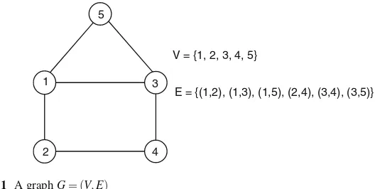
Agraphis a pairG= (V,E)consisting of a finite, nonempty setV of vertices and a setEofedges. Anedgeis an unordered pair of distinct vertices. (Forv_∈V,(v,v)

cannot be an edge because the vertices are not distinct.) If(u,v)is an edge, thenu andvare vertices; we say thatuandvareadjacent. A graph iscompleteif every pair of distinct vertices is connected by an edge.

AsubgraphofG= (V,E)is a graphG′= (V′,E′)such that 1. V′_⊆V, and

2. E′consists of edges(v,w)inEsuch that bothvandware inV′.

IfE′consists of all edges(v,w)inE such that bothvandware inV′, thenG′is called aninduced subgraphofG.

In most contexts(v,w)denotes an ordered pair, but when discussing graphs, we abuse notation by using(v,w)to denote edges, which are unordered pairs.

Apathis a sequence of vertices connected by edges. The length of a path is the number of edges on the path. (A single vertex is a path of length 0.) Asimple path is a path that does not repeat any vertex or edge, except possibly the first and last vertices. Acycleis a simple path of length at least 1 that starts and ends in the same vertex. Observe that the length of a cycle must be at least 3 becausevandu,v,uare not cycles. AHamiltonian circuitis a cycle that contains every vertex in the graph. Example 1.3. The sequence 1,2,4,3,5,1 is a Hamiltonian circuit of the graph in Fig.1.1.

A graph isconnectedif every two vertices has a path between them. The number of edges at a vertex is thedegreeof the vertex.

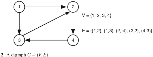
Adirected graph(digraph) consists of a set ofverticesand a set ofarcs. An arc is an ordered pair. Figure1.2gives an example.

A pathin a digraph is a sequence of vertices v1, . . . ,vn such that for everyi,

1≤i<n, there is an arc fromvitovi+1. A digraph isstrongly connectedif there is

a path from any vertex to any other vertex.

1

2

3

4 5

V = {1, 2, 3, 4, 5}

E = {(1,2), (1,3), (1,5), (2,4), (3,4), (3,5)}

1 2

3 4

V = {1, 2, 3, 4}

E = {(1,2), (1,3), (2, 4), (3,2), (4,3)}

Fig. 1.2 A digraphG= (V,E)

An (undirected)treeis a connected graph with no cycles.

For a directed graph we define a cycle just as for an undirected graph. Note that there can be cycles of length 2 in directed graphs. For directed graphs we define a tree as follows:

1. There is exactly one vertex, called the root, that no arcs enter; 2. Every other vertex is entered by exactly one arc; and

3. There is a path from the root to every vertex.

If(u,v)is an arc in a tree, thenuis aparentofv, andvis achildofu. If there is a path fromutov, thenuis anancestorofv, andvis adescendantofu. A vertex with no children is called aleaf. Avertex utogether with all its descendants is asubtree, anduis the root of that subtree.

Thedepthof a vertexuin a tree is the length of the path from the root tou. The heightofuis the length of a longest path fromuto a leaf. Theheight of the treeis the height of the root. Finally, when the children of each vertex are ordered, we call this anordered tree. Abinary treeis a tree such that each child of a vertex is either aleftchild or arightchild, and no vertex has more than one left child or right child.

1.5

Propositional Logic

Propositional logic provides a mathematical formalism that is useful for represent-ing and manipulatrepresent-ing statements of fact that are either true or false.

LetU={u1,u2,u3, . . .}be a set of Boolean variables (i.e., ranging over_{0,1_}, where we identify 0 with False and 1 with True). We associate the binary Boolean connectives_∧and_∨, and the unary connective_¬, with AND, inclusive-OR, and NOT, respectively. However, their exact semantic meaning will be given shortly. For now, they are purely syntactic.

The class ofpropositional formulasis defined inductively as follows: 1. Every propositional variable is a propositional formula;

2. IfAandBare propositional formulas, then the expressions(A_∧B),(A_∨B), and

When convenient, we will eliminate parentheses in propositional formulas in accordance with the usual precedence rules.

Definition 1.1. Let F be a propositional formula and let VAR(F) be the set of variables that occur inF. Anassignment(ortruth-assignment)tis a function

t: VAR(F)→ {0,1}.

An assignment induces a truth-value to the formulaFby induction, as follows: 1.

t((A_∧B)) =

1 ift(A) =t(B) =1; 0 otherwise.

2.

t((A_∨B)) =

0 ift(A) =t(B) =0; 1 otherwise.

3.

t((¬A)) =

1 ift(A) =0; 0 otherwise.

Using these rules, given any formulaF and an assignmentt to VAR(F), we can evaluatet(F)to determine whether the assignment makes the formula True or False. Also, these rules ascribe meaning to the connectives. It is common to present the truth-values of a formulaF under all possible assignments as a finite table, called a truth-table.

Ifu_∈Uis a Boolean variable, it is common to writeuin place of(¬u). Variables uand negated variablesuare calledliterals.

Example 1.4. The propositional formula (u1∨u2)∧(u1∨u2) has the following

truth-table:

u1u2(u1∨u2)∧(u1∨u2)

1 1 1

1 0 0

0 1 0

0 0 1

Definition 1.2. An assignmentt satisfiesa formulaF ift(F) =1. A formulaF is satisfiableif there exists an assignment to its variables that satisfies it.

We will learn in Chap.6 that the satisfiable formulas play an exceedingly important role in the study of complexity theory.

Definition 1.3. A formula is valid (or is a tautology) if every assignment to its variables satisfies it.

Proposition 1.1. A formula F is a tautology if and only if(¬F)is not satisfiable.

Definition 1.4. Two formulasF andGareequivalentif for every assignmentt to VAR(F)∪VAR(G),t(F) =t(G).

Next we define two special syntactic “normal” forms of propositional formulas. We will show that every formula is equivalent to one in each of these forms.

A formula is aconjunctionif it is of the form(A1∧A2∧ ···An), where eachAi

is a formula, and we often abbreviate this using the notation

1_≤i≤nAi. Similarly,

adisjunctionis a formula of the form(A1∨A2∨ ···An), which we can write as

1_≤i≤nAi.

A clause is a disjunction of literals. (For example, u1∨u3∨u8 is a clause.)

Observe that a clause is satisfied by an assignment if and only if the assignment makes at least one of its literals true.

Definition 1.5. A propositional formulaGis inconjunctive normal formif it is a conjunction of clauses.

Example 1.5. (u1∨u2)∧(u1∨u2)is in conjunctive normal form, the assignment

t(u1) =t(u2) =1 satisfies the formula, but it is not a tautology.

Example 1.6. (u1∧u1) is in conjunctive normal form and has no satisfying

assignment.

Homework 1.3 Show that every formula is equivalent to one in conjunctive

normal form. (You will need to use elementary laws of propositional logic such as DeMorgan’s laws, which state that_¬(A_∧B)is equivalent to(¬A_{∨ ¬}B)and that ¬(A_∨B)is equivalent to(¬A_{∧ ¬}B).)

Since a formula in conjunctive normal form is a conjunction of clauses, it is a conjunction of a disjunction of literals. Analogously, we define a formula to be in disjunctive normal formif it is a disjunction of a conjunction of literals.

Example 1.7. (u1∧u2)∨(u1∧u2)is in disjunctive normal form.

Using the technique of Homework1.3, every propositional formula is equivalent to one in disjunctive normal form.

1.5.1

Boolean Functions

ABoolean functionis a function f :{0,1}n_{→ {0,1}, wheren≥1. A truth-table}

is just a tabular presentation of a Boolean function, so every propositional formula defines a Boolean function by its truth-table.

Conversely, let f : {0,1}n _{→ {0,1} be a Boolean function. Then, we can}

represent f by the following formulaFf in disjunctive normal form whose

truth-table is f. For eachn-tuple(a1, . . . ,an)∈ {0,1}n_{such that f(a1, . . . ,an) =1, write}

the conjunction of literals(l1∧ ··· ∧ln), whereli=uiifai=1 andli=uiifai=0

(where 1≤i_≤n, andu1, . . . ,unare Boolean variables). Then, defineFf to be the

1.6

Cardinality

Thecardinalityof a set is a measure of its size. Two setsAandBhave thesame cardinalityif there is a bijectionh:A_→B. In this case we write card(A) =card(B). If there exists a one-to-one functionhfromAtoB, then card(A)≤card(B). For finite setsA={a1, . . . ,ak},k≥1, card(A) =k. A setAiscountableif card(A) =card(N)

orAis finite. A setAiscountably infiniteif card(A) =card(N).

A set isenumerableif it is the empty set or there is a function f :N_→ontoA. In

this caseAcan be written as a sequence: Writingaifor f(i), we have A=range(f) ={a0,a1,a2, . . .}={ai|i≥0}.

To call a set enumerable is to say that its elements can be counted. Observe that an enumeration need not be one-to-one. Sinceai=aj, fori= j, is possible, it is

possible that some elements ofAare counted more than once.

Theorem 1.2. A set is enumerable if and only if it is countable.

Homework 1.4 Prove Theorem1.2.

The cardinality ofNis denotedℵ0.

Theorem 1.3. A set A is countable if and only ifcard(A)≤ℵ0.

That is,ℵ0is the smallest nonfinite cardinality. (Of course, at the moment we

have no reason to expect that there is any other nonfinite cardinality.)

Proof. Suppose card(A)≤ℵ0. Then there is a one-to-one function f fromAtoN.

Suppose f[A]has a largest elementk. ThenAis a finite set. Suppose f[A]does not have a largest member. Leta0be the unique member ofA such that f(a0)is the

smallest member of f[A]. Letan+1be the unique member ofAsuch that f(an+1)is

the smallest member of f[A]− {f(a0), . . . ,f(an)}. It follows thatAis enumerable.

The reverse direction is straightforward. _⊓⊔

Homework 1.5 If card(A)≤card(B) and card(B)≤card(C), then card(A) ≤ card(C).

Homework 1.6 (This is a hard problem, known as the Cantor–Bernstein Theorem.)

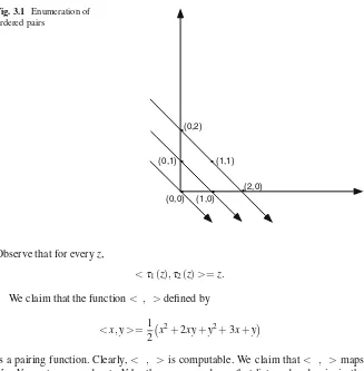
Ifcard(A)≤card(B)andcard(B)≤card(A), thencard(A) =card(B). Example 1.8. _{<x,y>|x,y_∈N_}is countable. An enumeration is

<0,0>, <0,1>, <1,0>, <0,2>, . . . .

Example 1.9. The set of rational numbers is countable.

Example 1.10. The set of programs in any programming language is countably infinite. For each language there is a finite alphabetΣ such that each program is inΣ∗_{. Because programs may be arbitrarily long, there are infinitely many of them.}

f_0(3) f_0(2)

f_0(1) f_0(0)

f_0

f_1(3) f_1(2)

f_1(1) f_1(0)

f_1

f_3(3) f_3(2)

f_3(1) f_3(0)

f_3

f_2(3) f_2(2)

f_2(1) f_2(0)

f_2

0 1 2 3

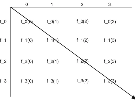
Fig. 1.3 The diagonalization technique

The proof of the following theorem employs the technique ofdiagonalization. Diagonalization was invented by the mathematician George Cantor (1845–1918), who created the theory of sets that we now take for granted. This is an important technique in theoretical computer science, so it would be wise to master this easy application first.

Theorem 1.4. The set of all functions from N to N is not countable.

Proof. Let A ={f _| f : N _→N_}. Suppose A is countable. Then there is an enumerationf0,f1, . . .ofA. (Think of all the values of each filaid out on an infinite

matrix: The idea is to define a function that cannot be on this matrix because it differs from all of the values on the diagonal. This is illustrated in Fig.1.3.) Define a functiongbyg(x) = fx(x) +1, for allx_∈N. Then,gis a function onN, but observe thatgcannot be in the enumeration of all functions. That is, ifg_∈A, then for some natural numberk,g=fk. Butgcannot equalfkbecauseg(k)=fk(k). Thus, we have

contradicted the assumption that the set of all functions can be enumerated. Thus,A

is not countable. _⊓⊔

Consider your favorite programming language. As there are countably many programs but there are uncountably many functions defined onN, there are functions that your favorite programming language cannot compute. All reasonable general-purpose programming systems compute the exact same set of functions, so it follows that there are functions defined onNthat are not computable by any program in any programming system.

For any setA,P_{(A) ={S|S⊆A}denotes the power set ofA.}

Proof. LetA=P₍N). Clearly,Ais infinite. Suppose A can be enumerated, and let S0,S1, . . . be an enumeration ofA. Then, defineT ={k_|k_∈S_k}. By definition,T belongs toA. However, for everyk,T =S_kbecausek_∈T _⇔k_∈S_k. Thus,T is a set that is not in the enumeration. So we have a contradiction. Thus,Acannot be

enumerated. ⊓⊔

1.6.1

Ordered Sets

It is useful to consider relations on the elements of a set that reflect the intuitive notion of ordering these elements.

Definition 1.6. A binary relationρon a setX is apartial orderif it is: 1. Reflexive(aρa, for alla_∈X),

2. Antisymmetric(aρbandbρaimpliesa=b, for allaandbinX), and 3. Transitive(aρbandbρcimpliesaρc, for alla,b, andcinX).

A partial order is a linear order on X if, in addition, for all a and b in X, aρborbρa.Apartially ordered set(linearly ordered set) is a pairX,ρ, where ρis a partial order (linear order, respectively) onX. LetZdenote the set of integers. Example 1.11. 1. Z,≤ and Z,≥ are linearly ordered sets, where ≤ and ≥

denote the customary well-known orderings onZ. 2. For any setA,P_{(A),⊆is a partially ordered set.}

3. Z,{(a,b)|a,b_∈Zandais an integral multiple ofb_}is a partially ordered set. 4. LetC _{be any collection of sets; then}

{card(X)|X_∈C_},≤

is a linear order.

1.7

Elementary Algebra

Here we present some useful algebra and number theory. In the next several pages we will barely scratch the surface of these exceedingly rich subjects. This material is not needed for the main body of the course, but is useful for understanding several examples in later chapters.

1.7.1

Rings and Fields

(A1) a+b=b+a(commutative law of addition);

(A2) (a+b) +c=a+ (b+c)(associative law of addition); (A3) a+0=a(zero element);

(A4) for everya_∈R, there existsx_∈Rsuch thata+x=0 (existence of additive inverses);

(A5) (ab)c=a(bc)1_{(associative law of multiplication);}

(A6) a(b+c) =ab+ac;

(A7) (b+c)a=ba+bc(distributive laws).

A ring iscommutativeif in addition it satisfies the following axiom: (A8) ab=ba(commutative law of multiplication).

A ring isring with unityif there is an element 1 belonging toRsuch that (A9) 1a=a1=a.

Definition 1.8. Afieldis a commutative ring with unityR,+,·,0,1such that (A10) for every a=0,a_∈R, there existsx_∈Rsuch thatax=1 (existence of

multiplicative inverses).

Note that 0 and 1 do not denote numbers – they are elements ofRthat obey the appropriate axioms.

Remember thatZdenotes the set of integers and letQdenote the set of all rational numbers. Then, using ordinary integer addition and multiplication and integers 0 and 1, Z forms a ring but not a field. The rational numbers Q, with its ordinary operations, forms a field.

Theorem 1.6. Each nonzero element in a field has a unique multiplicative inverse. Proof. Suppose thatsandtare two multiplicative inverses ofa. Then

s=s1=s(at) = (sa)t= (as)t=1t=t.

⊓ ⊔ The unique multiplicative inverse of an elementain a field is denoteda−1.

Definition 1.9. Letmbe an integer greater than 1 and letaandbbe integers. Then aiscongruent to b modulo mifmdividesa₋b.

We indicate thatmdividesa₋bby writingm_|a₋b, and we writea_≡b(modm)

to denote thatais congruent tobmodulom. Let rm(a,m)denote the remainder when dividingabym(eg., rm(5,2) =1).

Theorem 1.7. The following are elementary facts about congruence modulo m.

1. a_≡b (modm)if and only ifrm(a,m) =rm(b,m).

2.

a_≡b (modm)⇒ for all integers x, a+x_≡b+x(modm),

ax_≡bx(modm),and −a_{≡ −}b (modm).

3. Congruence modulo m is an equivalence relation.

Homework 1.7 Prove Theorem1.7.

Givenm>1, the equivalence class containing the integerais the set

[a] ={x_|x_≡a (modm)}.

We call[a]anequivalence class modulo m. LetZm denote the set of equivalence

classes modulo m, and let r=rm(a,m), so for some integer q, a=qm+r and 0_≤r<m. Then,a₋r=qm, soa_≡r (modm)and hence[a] = [r]. That is, every integer is congruent modulomto one of themintegers 0,1, . . . ,m₋1. Finally, no two of these are congruent modulom. Thus, there are exactlymequivalence classes modulom, and they are the sets [0],[1], . . . ,[m₋1]. We have learned that Zm = {[0],[1], . . .,[m₋1]}.

Now we will show thatZmforms a useful number system. We define operations

onZmas follows:[a] + [b] = [a+b]and[a][b] = [ab]. The definition is well founded,

i.e., independent of choice of representative member of each equivalence class, because

rm(a+b,m)≡rm(a,m) +rm(b,m) (modm)

and

rm(ab,m)≡rm(a,m)·rm(b,m) (modm).

We state the following theorem.

Theorem 1.8. For each positive integer m,Zm,+,·,[0],[1]is a ring with unity.

Homework 1.8 Prove the theorem by verifying each of the properties A1 to A8.

Definition 1.10. A commutative ring with unityR,+,·,0,1is anintegral domain if for alla,b_∈R,

(A11) ab=0 impliesa=0 orb=0 (absence of nontrivial zero divisors). The integers with their usual operations form an integral domain.

Theorem 1.9. Every field is an integral domain.

Proof. Suppose thatab=0. We show that ifa=0, then b=0, so suppose that a=0. Then the following holds:

b=1b=

a−1a

b=a−1(ab) =a−10=0.

Our goal is to show that ifpis a prime number, thenZpis a field. First, though, let

us observe that ifmis not a prime number, thenZmis not even an integral domain:

Namely, there exist positive integersa andb, 0<a<b<m, such that m=ab. Hence, inZm,[a][b] =0; yet[a]=0 and[b]=0.

To show thatZpis a field whenpis prime, we need to show that the equation

ax_≡1(modp)

is solvable2for each integera_{∈ {}1, . . . ,p₋1}. For this purpose, we introduce the following notation.

Definition 1.11. For nonzero integersa,b_∈Z, define

(a,b) ={ax+by_|x,y_∈Z_}

to be the set of alllinear combinationsofaandb, and define

(a) ={ax_|x_∈Z_}.

Definition 1.12. For nonzero integersa,b_∈Z, the positive integerd is agreatest common divisorofaandbif

(i) dis a divisor ofaandb, and

(ii) every divisor of bothaandbis a divisor ofd. We writed=gcd(a,b).

Lemma 1.1. (a,b) = (d), where d=gcd(a,b).

Proof. Sinceaandbare nonzero integers, there is a positive integer in(a,b). Letd be the least positive integer in(a,b). Clearly,(d)⊆(a,b).

We show (a,b)⊆(d): Supposec_∈(a,b). Then, there exist integers q and r such thatc=qd+r, with 0≤r<d. Sincecandd are in (a,b), it follows that r=c₋qd is in(a,b)also. However, since 0≤r<d andd is the least positive integer in(a,b), it must be the case thatr=0. Hence,c=qd, which belongs to(d). Thus,(d) = (a,b).

All that remains is to show thatd=gcd(a,b). Sinceaandb belong to(d),d is a common divisor of(a)and(b). Ifcis any other common divisor of(a)and

(b), thencdivides every number of the formax+by. Thus,c_|d, which proves that

d=gcd(a,b). ⊓⊔

Definition 1.13. Two integersaandbarerelatively primeif gcd(a,b) =1.

Theorem 1.10. If p is a prime number, thenZp,+,·,[0],[1]is a field.

Proof. Let[a]be a nonzero member ofZp. Then,[a]= [0], soa≡0 (mod p). That

is,pdoes not dividea. Thus, since pis prime,aandpare relatively prime. Now, let us apply Lemma1.1: There exist integersxandysuch that 1=ax+py. We can rewrite this as 1−ax=pyto see thatax_≡1(mod p). Hence,[a][x] = [1], which is

what we wanted to prove. ⊓⊔

Lemma1.1proves that the greatest common divisor of two integers always exists, but does not give a method of finding it. Next we present theEuclidean Algorithm, which computes gcd(x,y)for integersxandy. Later in the course we will analyze this algorithm to show that it is efficient.

Ifd=gcd(x,y), thendis the greatest common divisor of−xandy, ofxand−y, and of−xand−y, as well. Thus, in the following algorithm we assume thatxandy are positive integers.

EUCLIDEAN ALGORITHM

input positive integersxandyin binary notation;

repeat

x:=rm(x,y); exchangexandy

untily=0; outputx.

Let us understand the algorithm and see that it is correct. Letr1=rm(x,y), so

for some quotientq1,x=q1y+r1. Sincer1=x−q1y, every number that dividesx

andyalso dividesr1. Thus,d dividesr1, whered=gcd(x,y). Now we will show

that gcd(x,y) =gcd(y,r1). We know already thatd is a common divisor ofyand

r1. If there were a common divisord1>dthat dividesyandr1, then this valued1

would also dividex. Thus,dwould not be the greatest common divisor ofxandy. The Euclidean Algorithm reduces the problem of finding gcd(x,y) to that of finding gcd(y,r1), where r1<y. Since the remainder is always nonnegative and

keeps getting smaller, it must eventually be zero. Suppose this occurs after n iterations. Then we have the following system of equations:

x=q1y+r1,0<r1<y,

y=q2r1+r2,0<r2<r1,

r1=q3r2+r3,0<r3<r2,

r2=q4r3+r4,0<r4<r3,

.. .

rn−2=qnrn−1.

Finally,

andrn−1is the final value ofx, which completes the argument that the Euclidean

Algorithm computesd=gcd(x,y).

1.7.2

Groups

Definition 1.14. Agroupis a systemG,·,1that satisfies the following axioms, whereGis a nonempty set, 1 is an element ofG, and·is an operation onG: (A5) (ab)c=a(bc)

(A9) 1a=a1=a; and

(A12) for everya_∈Gthere existsx_∈Gsuch thatax=1.

A group iscommutativeif in addition it satisfies axiom (A8), the commutative law of multiplication.

The set of integersZforms a commutative groupZ,+,0known as theadditive group of the integers; for every positive integerm,Zm,+,[0]is a commutative

group. It follows from Theorem 1.10 that if p is a prime number, then Zp− {[0]},·,[1]is a commutative group. More generally, for every fieldF,+,·,0,1,, the nonzero elements ofF form a commutative groupF_{− {}0},·,1known as the multiplicative group of the field.

Definition 1.15. The order of a group G,·,1, written o(G), is the number of elements inGifGis finite, and is infinite otherwise.

Theorderof an elementainG,o(a), is the least positivemsuch thatam_{=1. If}

no such integer exists, theno(a)is infinite.

The order of the additive group of the integers is infinite. The order of the additive groupZm,+,[0]ism, while, forpa prime, the order of the multiplicative group of

the nonzero elements ofZpisp−1.

Definition 1.16. LetHbe a nonempty subset ofG.His asubgroupofG(or more preciselyH,·,1is asubgroupofG,·,1) ifHcontains the identity element 1 and H,·,1is a group.

LetG,·,1be a group anda_∈G. Then the setH={ai_|i_∈Z_}is a subgroup ofG. We claim that H containso(a)many elements. Of course, ifH is infinite, theno(a)is infinite. Suppose thatH is finite, and leto(a) =m. Letak_∈H. Then for some integerqand 0≤r<m,ak=aqm+r = (am)q_ar_=1ar_=ar_.Thus,H= {1,a, . . .,am−1_}, soHcontains at mosto(a)elements. Ifo(H)<o(a), then for some iandj, 0≤i<j<o(a),ai=aj. Hence,aj−i=1. However,j₋i<o(a), which is a contradiction. Thus,o(H) =o(a).

For any groupG,·,1anda_∈G,H={ai_|i_∈Z_}is a cyclic subgroup ofGand ais a generator of the subgroup.

1.7.2.1 Cosets

Now we come to a remarkable point: Every subgroupHof a groupGpartitionsG into disjoint cosets.

Definition 1.18. Given a subgroupHof a groupGand elementa_∈G, defineaH= {ah_|h_∈H_}. The setaHis called acosetofH.

The following lemma lists the basic properties of cosets.

Lemma 1.2. Let a and b be members of a group G and let H be a subgroup of G. 1. aH_∩bH=/0implies aH=bH.

2. For finite subgroups H, aH contains o(H)many elements.

Proof. Suppose that aH and bH have an elementc=ah′=bh′′ (h′,h′′ _∈H) in common. Leth_∈H. Then,bh=bh′′h′′−1h=a(h′h′′−1h), which belongs toaH. Thus,aH_⊆bH. Similarly,bHcontains every element ofaH, and soaH=bH.

To see thataHhaso(H)many elements, we note that the mappingh_→ah(from HtoaH) is one-to-one: Each elementx=ah,h_∈H, in the cosetaH is the image of the unique elementh=a−1x. _⊓⊔ The elementa=a1_∈aH. Thus, every element ofG belongs to some coset, and because distinct cosets are disjoint, every element of Gbelongs to a unique coset. The cosets ofH partitionG. Thus, the proof of the next theorem follows immediately.

Theorem 1.11 (Lagrange). Let H be a subgroup of a finite group G. Then,

o(H)|o(G).

Lagrange’s theorem has several important corollaries.

Corollary 1.1. If G is a finite group and a_∈G, then ao(G)=1. Proof. For some nonzero integern,o(G) =n_·o(a), so

ao(G)=an·o(a)= (ao(a))n₌₁n_=1.

⊓ ⊔

Corollary 1.2. Every group of order p, where p is prime, is a cyclic group. As a consequence, for each prime p, the additive groupZp,+,[0]is a cyclic

group.

We apply Corollary1.1to the multiplicative groupZp− {[0]},·,[1]to obtain

Corollary 1.3 (Fermat). If a is an integer, p is prime, and p does not divide a, then ap−1_≡1(mod p).

1.7.3

Number Theory

Our goal is to show that the multiplicative group of the nonzero elements of a finite field is a cyclic group. We know from Corollary1.3that for each prime number pand integera, 1≤a_≤p₋1,ap−1_{≡1 (modp). However, we do not yet know}

whether there is a generatorg, 1≤g_≤p₋1, such that p₋1 is the leastpower msuch thatgm_{≡1 (mod p). This is the result that will conclude this section. We}

begin with the following result, known as theChinese Remainder Theorem.

Theorem 1.12 (Chinese Remainder Theorem). Let m1, . . . ,mkbe pairwise rela-tively prime positive integers; that is, for all i and j,1≤i,j_≤k, i= j,gcd(mi,mj) =

1. Let a1, . . . ,ak be arbitrary integers. Then there is an integer x that satisfies the following system of simultaneous congruences:

x_≡a1(modm1)

x_≡a2(modm2)

.. .

x_≡ak(modmk).

Furthermore, there is a unique solution in the sense that any two solutions are congruent to one another modulo the value M=m1m2···mk.

Proof. For everyi, 1_≤i_≤k, defineMi=M/mi. Then, clearly, gcd(mi,Mi) =1. By

Lemma1.1, there existcianddisuch thatciMi+d1mi=1, sociMi≡1 (modmi).

Takex=∑iaiciMi. For any i, consider theith term of the sum: For each j=i, mi|Mj. Thus, every term in the sum other than theith term is divisible bymi. Hence, x_≡aiciMi≡ai (modmi), which is what we needed to prove.

Now we prove uniqueness moduloM. Suppose thatxandy are two different solutions to the system of congruences. Then, for each i,x₋y_≡0(modmi). It follows thatx₋y_≡0 (modM), and this completes the proof. _⊓⊔ The Eulerphi-functionφ(m)is defined to be the number of integers less thanm that are relatively prime tom. If pis a prime, thenφ(p) =p₋1.

Theorem 1.13. If m and n are relatively prime positive integers, then φ(mn) = φ(m)φ(n).

Proof. We computeφ(mn). For each 1_≤i<mn, letr1be the remainder of dividing

ibymand letr2be the remainder of dividingibyn. Then 0≤r1<m, 0≤r2<n,

Chinese Remainder Theorem, there is exactly one valuei, 1_≤i<mn, such thati_≡ r1(modm)andi≡r2 (modn). Consider this one-to-one correspondence between

integers 1_≤i<mnand pairs of integers(r1,r2), 0≤r1<m, 0≤r2<n, such that

i_≡r1(modm)andi≡r2(modn): Note thatiis relatively prime tomnif and only

ifiis relatively prime tomandiis relatively prime ton. This occurs if and only ifr1

is relatively prime tomandr2is relatively prime ton. The number of suchiisφ(mn),

while the number of such pairs(r1,r2)isφ(m)φ(n). Thus,φ(mn) =φ(m)φ(n). ⊓⊔

Let the prime numbers in increasing order be

p1=2,p2=3,p3=5, . . . .

Every positive integerahas a unique factorization as a product of powers of primes of the form

not relatively prime topa_{. It follows that there are}

φ(pa) = (pa₋1)−(pa−1₋1) = (pa₋pa−1)

positive integers less thanpa_{that are relatively prime top}a_.

We define a function f on the positive integers by f(n) =∑d_|nφ(d). We need to

Lemma 1.4. If m and n are relatively prime positive integers, then f(mn) =

f(m)f(n).

Proof. Every divisordofmncan be written uniquely as a productd=d1d2, where

d1is a divisor ofmandd2is a divisor ofn. Conversely, for every divisord1ofmand

d2ofn,d=d1d2is a divisor ofmn. Note thatd1andd2are relatively prime. Thus,

f(mn) =

_∑

d|mn

φ(d)

=

_∑

d1|md

∑

2|n

φ(d1)φ(d2)

=

_∑

d1|m

φ(d1)

∑

d2|n

φ(d2)

= f(m)f(n).

⊓ ⊔

Theorem 1.14. For every positive integer n,∑d_|nφ(d) =n.

Proof. The integern is a product of relatively prime terms of the formpa, so the proof follows immediately from Lemmas1.3and1.4. ⊓⊔

1.7.3.1 Polynomials

LetF,+,·,0,1be a field and letxbe a symbol. The expression

k

∑

0

akxk,

where the coefficients ai, i≤k, belong to F, is a polynomial. The degree of a

polynomial is the largest numberksuch that the coefficientak=0; this coefficient is

called theleadingcoefficient. One adds or multiplies polynomials according to the rules of high school algebra. With these operations the set of all polynomials overF forms apolynomial ring F[x]. We say thatg divides f, where f,g_∈F[x], if there is a polynomialh_∈F[x]such that f=gh. An elementa_∈Fis arootof a polynomial

f(x)∈F[x]if f(a) =0.

Homework 1.9 Verify that F[x]is a ring.

Theorem 1.15. If f(x),g(x)∈F[x], g(x)is a polynomial of degree n, the leading coefficient of g(x) is 1, and f(x) is of degree m_≥n, then there exist unique polynomials q(x)and r(x)in F[x]such that f(x) =q(x)g(x) +r(x), and r(x) =0or the degree of r(x)is less than the degree of g(x).

The proof proceeds by applying thedivision algorithm, which we now sketch: Suppose that f(x) =∑m0amxm. We can make the leading coefficientam vanish by

subtracting from f a multiple ofg, namely,amxm−ng(x). After this subtraction, if

Lemma 1.5. If a is a root of f(x)∈F[x], then f(x)is divisible by x₋a.

Proof. Applying the division algorithm, we get f(x) =q(x)(x₋a) +r, wherer_∈F is a constant. Substituteafor thexto see that 0= f(a) =q(a)·0+r=r. Thus,

f(x) =q(x)(x₋r). ⊓⊔

Theorem 1.16. If a1, . . . ,a_kare different roots of f(x), then f(x)is divisible by the product(x₋a1)(x−a2)···(x−ak).

The proof is by mathematical induction in which Lemma1.5provides the base casek=1.

Corollary 1.4. A polynomial in F[x] of degree n that is distinct from zero has at most n roots in F.

This concludes our tutorial on polynomials. We turn now to show that the multiplicative group of the nonzero elements of a finite field is cyclic.

Let F,+,·,0,1 be a finite field with q elements. Then the multiplicative subgroup of nonzero elements ofF has orderq₋1. Our goal is to show that this group has a generatorgof orderq₋1. By Lagrange’s theorem, Theorem1.11, we know that the order of every nonzero elementainF is a divisor ofq₋1. Our first step is to show that for every positive integerd_|(q₋1), there are either 0 orφ(d)

nonzero elements inFof orderd.

Lemma 1.6. For every d_|(q₋1), there are either 0 orφ(d)nonzero elements in F of order d.

Proof. Letd_|(q₋1), and suppose that some elementahas orderd. We will show that there must beφ(d)elements of orderd. By definition, each of the elements a,a2, . . . ,ad=1 is distinct. Each of these powers ofa is a root of the polynomial xd₋1. Thus, by Corollary 1.4, since every element of orderd is a root of this polynomial, every element of orderdmust be among the powers ofa. Next we will show thataj, 1≤j<d, has orderdif and only if gcd(j,d) =1. From this, it follows immediately that there areφ(d)elements of orderd.

Let gcd(j,d) =1, where 1≤j<d, and suppose thataj has orderc<d. Then

(ac)j_{= (a}j₎c_{=1 and(a}c₎d_{= (a}d₎c_{=1. By Lemma1.1, sincejanddare relatively}

prime, there are integersuandvsuch that 1=u j+vd. Clearly, one of these integers must be positive and the other negative. Assume thatu>0 andv_≤0. Then(ac)u j₌

1 and(ac)−vd _{=1, so dividing on both sides, we geta}c_{= (a}c₎u j+vd_{=1. However,}

sincec<d, this contradicts the fact thato(a) =d. Thus, our supposition thato(aj)<

dis false;ajhas orderd.

Conversely, suppose that gcd(j,d) =d′>1. Thend/d′and j/d′are integers, so

(aj)d/d′ _{= (a}d₎j/d′_{=1. Thus,o(a}j_)≤d/d′_<d.

This completes the proof. _⊓⊔

Proof. Let F,+,·,0,1 be a finite field with q elements. We need to show that the multiplicative groupF_{− {}0},+,·,1has a generator, an element a of order q₋1. Every elementahas some orderd such thatd_|(q₋1), and by Lemma1.6, for every suchd, there are either 0 orφ(d)nonzero elements inF of orderd. By Theorem1.14,∑d_|(q−1)φ(d) =q−1, which is the number of elements inF− {0}.

Hence, in order for every element to have some orderdthat is a divisor ofq₋1, it must be the case for every suchd that there areφ(d)many elements of orderd. In particular, there areφ(q₋1)different elementsg_∈Fof orderq₋1. Thus, there is a generator, and the multiplicative group of nonzero elements ofFis cyclic. ⊓⊔

Corollary 1.5. If p is a prime number, thenZp− {[0]},·,[1]is a cyclic group.

For example, the number 2 is a generator ofZ19. Namely, the powers of 2 modulo

19 are 2, 4, 8, 16, 13, 7, 14, 9, 18, 17, 15, 11, 3, 6, 12, 5, 10, 1.

Homework 1.10 What are the other generators for Z19?

Once considered to be the purest branch of mathematics, devoid of application, number theory is the mathematical basis for the security of electronic commerce, which is fast becoming an annual trillion-dollar industry. Modern cryptography depends on techniques for finding large prime numbers p and generators for Zp