Elliptic Curves Number Theory and Cryptography,

E l l i p t ic C u rv e s

Number Theory

and Cryptography

-*!'#**-*)/-* 0/%*)/** %)#$!*-4

*'#'%'",*#'#*-%/$(%*(%)/*-%.*)-/%'*- .

-'("(''!-+))%)#-!!.) +/%(%5/%*)-*'!(.

"*%&(+"*%&#+)0(!-/%1!*(%)/*-%.

'*#("'*"**1,%) **&*"''%+/%) 4+!-!''%+/%0-1!-4+/*#-+$4 "*%+(%(-*'' *1#'#,2) **&*"*(%)/*-%' !.%#).!*) %/%*) *,#' *#$+(''',"('122')/-* 0/%*)/*0(!-$!*-4

,.'-*#'(#'!#('#'0#'!#'-(!.) !.*'1'! !.%#)..!.

*)./-0/%*).) 3%./!)!

'1(%*!''#$-/%') **&*"+!!$* !-.

( ((&''(+)"4(-*$) **&*" %.-!/!) *(+0//%*)'!*(!/-4 !*) %/%*)

(',"'*(++*(%)/*-%'!/$* .2%/$*(+0/!-++'%/%*).

(',"'*(++'1%%'-+$$!*-4) /.++'%/%*).!*) %/%*) (',"'*(++'1%%') **&*"-+$$!*-4

**%'$*+('*!**#+',*("'+(')/-* 0/%*)/*)"*-(/%*) $!*-4) /*(+-!..%*)!*) %/%*)

*1%*&+#*(+%.*,2%"*%+(%(-*''("'.#,,!/2*-&!'%%'%/4 3+!-%(!)/.2%/$4(*'%'#!-)1%-*)(!)/

+%#(!')

**&*"%)!-'#!-*$(%,/#,",,#' #$' &(''4*#') **&*"*(+0//%*)'-*0+$!*-4

.#$+(''**1#+',#')/'.*"(''!-+.%)-%!)/'!)

*)*-%!)/'!0-"!.

#"* %#&#% #!&('' *'+,,#,2#'!* ++'%/%*).*"./-/'#!-2%/$+'!7) 6!*) %/%*)

,*#$'-))'&#2%*#!-%"%/%*)*"*(+0/!-* !.%)*(+0//%*)'%!)! ) )#%)!!-%)#

!-%!.

%/*-!))!/$*.!)$

DISCRETE

MATHEMATICS

#%%#&(1'('%*"*-+$.'#*-%/$(.) +/%(%5/%*)

('%*"*'(-!%+,#'+('*(%)/*-%''#*-%/$(.!)!-/%*))0(!-/%*) ) !-$

"*%+#''*'"*#+,()"*(!*+ !.%#)$!*-4 '!-1%--4*"-+$'#*-%/$(.) +/%(%5/%*)

% *'2+-%.'(*+"(,'(,,'+,(') **&*"++'%! -4+/*#-+$4

#"*(%%#''#!-%0(!-$!*-4

#"*(%%#'* !.$!0% !/*!-!4"-*()%!)//** !-)%(!. #"*(%%#'0) (!)/'0(!-$!*-42%/$++'%/%*).!*) %/%*) #"*(%%#'))/-* 0/%*)/*-4+/*#-+$4!*) %/%*)

#"*(%%#'0 -/%.

#"*(%%#') 0'%!4-4+/*#-+$4

*%(+(*'('&-%!+, *0(.*",0-!.*")/!#!-. #'!1##0/$!)/%/%*)* !.) *(%)/*-%' !.%#).

'',"(+') **&*" %.-!/!) *(%)/*-%'/$!(/%.

(-!%+"#*'%%'#-+++'%! /$!(/%'* !'%)#0'/% %.%+'%)-4 ++-*$

3*',-#'! %*+$)/%)!)'4.%.

(-!%+,#'+('-4+/*#-+$4$!*-4) -/%!$%- %/%*)

(*,((!'*#'"*#+,()"*#%.0) (!)/'.*")"*-(/%*)$!*-4) * %)# !.%#)

%%#+)/-* 0/%*)/**(%)/*-%' !.%#).!*) %/%*)

Series Editor KENNETH H. ROSEN

L AW R E NC E C . WA S H I NG TON

Uni v e r si t y of M a ry l a nd

C ol l e g e Pa r k , M a ry l a nd , U . S . A .

E l l i p t ic C u rv e s

Number Theory

and Cryptography

6000 Broken Sound Parkway NW, Suite 300 Boca Raton, FL 33487-2742

© 2008 by Taylor & Francis Group, LLC

Chapman & Hall/CRC is an imprint of Taylor & Francis Group, an Informa business

No claim to original U.S. Government works

Printed in the United States of America on acid-free paper 10 9 8 7 6 5 4 3 2 1

International Standard Book Number-13: 978-1-4200-7146-7 (Hardcover)

This book contains information obtained from authentic and highly regarded sources Reason-able efforts have been made to publish reliReason-able data and information, but the author and publisher cannot assume responsibility for the validity of all materials or the consequences of their use. The Authors and Publishers have attempted to trace the copyright holders of all material reproduced in this publication and apologize to copyright holders if permission to publish in this form has not been obtained. If any copyright material has not been acknowledged please write and let us know so we may rectify in any future reprint

Except as permitted under U.S. Copyright Law, no part of this book may be reprinted, reproduced, transmitted, or utilized in any form by any electronic, mechanical, or other means, now known or hereafter invented, including photocopying, microfilming, and recording, or in any information storage or retrieval system, without written permission from the publishers.

For permission to photocopy or use material electronically from this work, please access www. copyright.com (http://www.copyright.com/) or contact the Copyright Clearance Center, Inc. (CCC) 222 Rosewood Drive, Danvers, MA 01923, 978-750-8400. CCC is a not-for-profit organization that provides licenses and registration for a variety of users. For organizations that have been granted a photocopy license by the CCC, a separate system of payment has been arranged.

Trademark Notice: Product or corporate names may be trademarks or registered trademarks, and are used only for identification and explanation without intent to infringe.

Library of Congress Cataloging-in-Publication Data

Washington, Lawrence C.

Elliptic curves : number theory and cryptography / Lawrence C. Washington. -- 2nd ed.

p. cm. -- (Discrete mathematics and its applications ; 50) Includes bibliographical references and index.

ISBN 978-1-4200-7146-7 (hardback : alk. paper)

1. Curves, Elliptic. 2. Number theory. 3. Cryptography. I. Title. II. Series.

QA567.2.E44W37 2008

516.3’52--dc22 2008006296

Visit the Taylor & Francis Web site at http://www.taylorandfrancis.com

Over the last two or three decades, elliptic curves have been playing an in-creasingly important role both in number theory and in related fields such as cryptography. For example, in the 1980s, elliptic curves started being used in cryptography and elliptic curve techniques were developed for factorization and primality testing. In the 1980s and 1990s, elliptic curves played an impor-tant role in the proof of Fermat’s Last Theorem. The goal of the present book is to develop the theory of elliptic curves assuming only modest backgrounds in elementary number theory and in groups and fields, approximately what would be covered in a strong undergraduate or beginning graduate abstract algebra course. In particular, we do not assume the reader has seen any al-gebraic geometry. Except for a few isolated sections, which can be omitted if desired, we do not assume the reader knows Galois theory. We implicitly use Galois theory for finite fields, but in this case everything can be done explicitly in terms of the Frobenius map so the general theory is not needed. The relevant facts are explained in an appendix.

The book provides an introduction to both the cryptographic side and the number theoretic side of elliptic curves. For this reason, we treat elliptic curves over finite fields early in the book, namely in Chapter 4. This immediately leads into the discrete logarithm problem and cryptography in Chapters 5, 6, and 7. The reader only interested in cryptography can subsequently skip to Chapters 11 and 13, where the Weil and Tate-Lichtenbaum pairings and hy-perelliptic curves are discussed. But surely anyone who becomes an expert in cryptographic applications will have a little curiosity as to how elliptic curves are used in number theory. Similarly, a non-applications oriented reader could skip Chapters 5, 6, and 7 and jump straight into the number theory in Chap-ters 8 and beyond. But the cryptographic applications are interesting and provide examples for how the theory can be used.

present book, but contains few proofs. It should be consulted by serious stu-dents of elliptic curve cryptography. We hope that the present book provides a good introduction to and explanation of the mathematics used in that book. The books by Enge [38], Koblitz [66], [65], and Menezes [82] also treat elliptic curves from a cryptographic viewpoint and can be profitably consulted.

Notation.

The symbols Z, Fq, Q, R, C denote the integers, the finite

field with q elements, the rationals, the reals, and the complex numbers, respectively. We have used Zn (rather than Z/nZ) to denote the integers

mod n. However, when p is a prime and we are working with Zp as a field,

rather than as a group or ring, we use Fp in order to remain consistent with

the notation Fq. Note that Zp does not denote the p-adic integers. This

choice was made for typographic reasons since the integers mod p are used frequently, while a symbol for thep-adic integers is used only in a few examples in Chapter 13 (where we use _Op). The p-adic rationals are denoted by Qp.

IfK is a field, then K denotes an algebraic closure of K. If R is a ring, then R× _{denotes the invertible elements of R. When K is a field, K}× _{is therefore} the multiplicative group of nonzero elements of K. Throughout the book, the letters K and E are generally used to denote a field and an elliptic curve (except in Chapter 9, where K is used a few times for an elliptic integral).

The main question asked by the reader of a preface to a second edition is “What is new?” The main additions are the following:

1. A chapter on isogenies.

2. A chapter on hyperelliptic curves, which are becoming prominent in many situations, especially in cryptography.

3. A discussion of alternative coordinate systems (projective coordinates, Jacobian coordinates, Edwards coordinates) and related computational issues.

4. A more complete treatment of the Weil and Tate-Lichtenbaum pairings, including an elementary definition of the Tate-Lichtenbaum pairing, a proof of its nondegeneracy, and a proof of the equality of two common definitions of the Weil pairing.

5. Doud’s analytic method for computing torsion on elliptic curves overQ. 6. Some additional techniques for determining the group of points for an

elliptic curve over a finite field.

7. A discussion of how to do computations with elliptic curves in some popular computer algebra systems.

8. Several more exercises.

This book is intended for at least two audiences. One is computer scientists and cryptographers who want to learn about elliptic curves. The other is for mathematicians who want to learn about the number theory and geometry of elliptic curves. Of course, there is some overlap between the two groups. The author of course hopes the reader wants to read the whole book. However, for those who want to start with only some of the chapters, we make the following suggestions.

Everyone: A basic introduction to the subject is contained in Chapters 1, 2, 3, 4. Everyone should read these.

I. Cryptographic Track: Continue with Chapters 5, 6, 7. Then go to Chapters 11 and 13.

II. Number Theory Track: Read Chapters 8, 9, 10, 11, 12, 14, 15. Then go back and read the chapters you skipped since you should know how the subject is being used in applications.

1 Introduction 1

Exercises . . . 8

2 The Basic Theory 9 2.1 Weierstrass Equations . . . 9

2.2 The Group Law . . . 12

2.3 Projective Space and the Point at Infinity . . . 18

2.4 Proof of Associativity . . . 20

2.4.1 The Theorems of Pappus and Pascal . . . 33

2.5 Other Equations for Elliptic Curves . . . 35

2.5.1 Legendre Equation . . . 35

2.5.2 Cubic Equations . . . 36

2.5.3 Quartic Equations . . . 37

2.5.4 Intersection of Two Quadratic Surfaces . . . 39

2.6 Other Coordinate Systems . . . 42

2.6.1 Projective Coordinates . . . 42

2.6.2 Jacobian Coordinates . . . 43

2.6.3 Edwards Coordinates . . . 44

2.7 The j-invariant . . . 45

2.8 Elliptic Curves in Characteristic 2 . . . 47

2.9 Endomorphisms . . . 50

2.10 Singular Curves . . . 59

2.11 Elliptic Curves mod n . . . 64

Exercises . . . 71

3 Torsion Points 77 3.1 Torsion Points . . . 77

3.2 Division Polynomials . . . 80

3.3 The Weil Pairing . . . 86

3.4 The Tate-Lichtenbaum Pairing . . . 90

Exercises . . . 92

4 Elliptic Curves over Finite Fields 95 4.1 Examples . . . 95

4.2 The Frobenius Endomorphism . . . 98

4.3 Determining the Group Order . . . 102

4.3.2 Legendre Symbols . . . 104

4.3.3 Orders of Points . . . 106

4.3.4 Baby Step, Giant Step . . . 112

4.4 A Family of Curves . . . 115

4.5 Schoof’s Algorithm . . . 123

4.6 Supersingular Curves . . . 130

Exercises . . . 139

5 The Discrete Logarithm Problem 143 5.1 The Index Calculus . . . 144

5.2 General Attacks on Discrete Logs . . . 146

5.2.1 Baby Step, Giant Step . . . 146

5.2.2 Pollard’s ρ and λ Methods . . . 147

5.2.3 The Pohlig-Hellman Method . . . 151

5.3 Attacks with Pairings . . . 154

5.3.1 The MOV Attack . . . 154

5.3.2 The Frey-R¨uck Attack . . . 157

5.4 Anomalous Curves . . . 159

5.5 Other Attacks . . . 165

Exercises . . . 166

6 Elliptic Curve Cryptography 169 6.1 The Basic Setup . . . 169

6.2 Diffie-Hellman Key Exchange . . . 170

6.3 Massey-Omura Encryption . . . 173

6.4 ElGamal Public Key Encryption . . . 174

6.5 ElGamal Digital Signatures . . . 175

6.6 The Digital Signature Algorithm . . . 179

6.7 ECIES . . . 180

6.8 A Public Key Scheme Based on Factoring . . . 181

6.9 A Cryptosystem Based on the Weil Pairing . . . 184

Exercises . . . 187

7 Other Applications 189 7.1 Factoring Using Elliptic Curves . . . 189

7.2 Primality Testing . . . 194

Exercises . . . 197

8 Elliptic Curves over Q 199 8.1 The Torsion Subgroup. The Lutz-Nagell Theorem . . . 199

8.2 Descent and the Weak Mordell-Weil Theorem . . . 208

8.3 Heights and the Mordell-Weil Theorem . . . 215

8.4 Examples . . . 223

8.5 The Height Pairing . . . 230

8.7 2-Selmer Groups; Shafarevich-Tate Groups . . . 236

8.8 A Nontrivial Shafarevich-Tate Group . . . 239

8.9 Galois Cohomology . . . 244

Exercises . . . 253

9 Elliptic Curves over C 257 9.1 Doubly Periodic Functions . . . 257

9.2 Tori are Elliptic Curves . . . 267

9.3 Elliptic Curves over C . . . 272

9.4 Computing Periods . . . 286

9.4.1 The Arithmetic-Geometric Mean . . . 288

9.5 Division Polynomials . . . 294

9.6 The Torsion Subgroup: Doud’s Method . . . 302

Exercises . . . 307

10 Complex Multiplication 311 10.1 Elliptic Curves over C . . . 311

10.2 Elliptic Curves over Finite Fields . . . 318

10.3 Integrality of j-invariants . . . 322

10.4 Numerical Examples . . . 330

10.5 Kronecker’s Jugendtraum . . . 336

Exercises . . . 337

11 Divisors 339 11.1 Definitions and Examples . . . 339

11.2 The Weil Pairing . . . 349

11.3 The Tate-Lichtenbaum Pairing . . . 354

11.4 Computation of the Pairings . . . 358

11.5 Genus One Curves and Elliptic Curves . . . 364

11.6 Equivalence of the Definitions of the Pairings . . . 370

11.6.1 The Weil Pairing . . . 371

11.6.2 The Tate-Lichtenbaum Pairing . . . 374

11.7 Nondegeneracy of the Tate-Lichtenbaum Pairing . . . 375

Exercises . . . 379

12 Isogenies 381 12.1 The Complex Theory . . . 381

12.2 The Algebraic Theory . . . 386

12.3 V´elu’s Formulas . . . 392

12.4 Point Counting . . . 396

12.5 Complements . . . 401

13 Hyperelliptic Curves 407

13.1 Basic Definitions . . . 407

13.2 Divisors . . . 409

13.3 Cantor’s Algorithm . . . 417

13.4 The Discrete Logarithm Problem . . . 420

Exercises . . . 426

14 Zeta Functions 429 14.1 Elliptic Curves over Finite Fields . . . 429

14.2 Elliptic Curves over Q . . . 433

Exercises . . . 442

15 Fermat’s Last Theorem 445 15.1 Overview . . . 445

15.2 Galois Representations . . . 448

15.3 Sketch of Ribet’s Proof . . . 454

15.4 Sketch of Wiles’s Proof . . . 461

A Number Theory 471 B Groups 477 C Fields 481 D Computer Packages 489 D.1 Pari . . . 489

D.2 Magma . . . 492

D.3 SAGE . . . 494

Chapter 1

Introduction

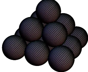
Suppose a collection of cannonballs is piled in a square pyramid with one ball on the top layer, four on the second layer, nine on the third layer, etc. If the pile collapses, is it possible to rearrange the balls into a square array?

Figure 1.1

A Pyramid of Cannonballs

If the pyramid has three layers, then this cannot be done since there are 1 + 4 + 9 = 14 balls, which is not a perfect square. Of course, if there is only one ball, it forms a height one pyramid and also a one-by-one square. If there are no cannonballs, we have a height zero pyramid and a zero-by-zero square. Besides theses trivial cases, are there any others? We propose to find another example, using a method that goes back to Diophantus (around 250 A.D.).

If the pyramid has height x, then there are

12+ 22+ 32+_{· · ·}+x2= x(x+ 1)(2x+ 1) 6

balls (see Exercise 1.1). We want this to be a perfect square, which means that we want to find a solution to

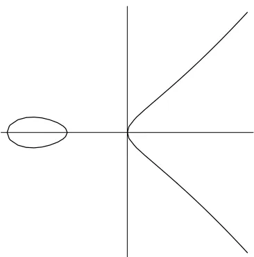
Figure 1.2

y2_{=x(x+ 1)(2x+ 1)/6}

in positive integersx, y. An equation of this type represents anelliptic curve. The graph is given in Figure 1.2.

The method of Diophantus uses the points we already know to produce new points. Let’s start with the points (0,0) and (1,1). The line through these two points is y =x. Intersecting with the curve gives the equation

x2 = x(x+ 1)(2x+ 1)

6 =

1 3x

3₊ 1

2x

2₊ 1

6x. Rearranging yields

x3₋ 3 2x

2₊ 1

2x= 0.

Fortunately, we already know two roots of this equation: x = 0 and x = 1. This is because the roots are the x-coordinates of the intersections between the line and the curve. We could factor the polynomial to find the third root, but there is a better way. Note that for any numbersa, b, c, we have

(x₋a)(x₋b)(x₋c) = x3₋(a+b+c)x2+ (ab+ac+bc)x₋abc. Therefore, when the coefficient ofx3 is 1, the negative of the coefficient of x2 is the sum of the roots.

In our case, we have roots 0,1, and x, so

0 + 1 +x= 3 2.

Let’s repeat the above procedure using the points (1/2,₋1/2) and (1,1). Why do we use these points? We are looking for a point of intersection somewhere in the first quadrant, and the line through these two points seems to be the best choice. The line is easily seen to be y = 3x₋2. Intersecting with the curve yields

(3x₋2)2 = x(x+ 1)(2x+ 1)

6 .

This can be rearranged to obtain

x3₋ 51 2 x

2₊

· · ·= 0.

(By the above trick, we will not need the lower terms.) We already know the roots 1/2 and 1, so we obtain

1

2 + 1 +x= 51

2 ,

or x= 24. Since y = 3x₋2, we find that y = 70. This means that

12+ 22+ 32+_{· · ·}+ 242= 702.

If we have 4900 cannonballs, we can arrange them in a pyramid of height 24, or put them in a 70-by-70 square. If we keep repeating the above procedure, for example, using the point just found as one of our points, we’ll obtain infinitely many rational solutions to our equation. However, it can be shown that (24, 70) is the only solution to our problem in positive integers other than the trivial solution with x = 1. This requires more sophisticated techniques and we omit the details. See [5].

Here is another example of Diophantus’s method. Is there a right triangle with rational sides with area equal to 5? The smallest Pythagorean triple (3,4,5) yields a triangle with area 6, so we see that we cannot restrict our attention to integers. Now look at the triangle with sides (8, 15, 17). This yields a triangle with area 60. If we divide the sides by 2, we end up with a triangle with sides (4, 15/2, 17/2) and area 15. So it is possible to have nonintegral sides but integral area.

Let the triangle we are looking for have sides a, b, c, as in Figure 1.3. Since the area is ab/2 = 5, we are looking for rational numbers a, b, c such that

a2+b2 =c2, ab= 10. A little manipulation yields

a+b 2

2

= a

2_{+ 2ab+b}2

4 =

c2_{+ 20}

4 =

_c

2

2

+ 5,

a₋b 2

2

= a

2_−2ab+b2

4 =

c2₋₂₀

4 =

_c

2

2

a

b

c

Figure 1.3

Let x= (c/2)2. Then we have

x₋5 = ((a₋b)/2)2 and x+ 5 = ((a+b)/2)2. We are therefore looking for a rational numberx such that

x₋5, x, x+ 5

are simultaneously squares of rational numbers. Another way to say this is that we want three squares of rational numbers to be in an arithmetical progression with difference 5.

Suppose we have such a number x. Then the product (x₋5)(x)(x+ 5) = x3_{−25x must also be a square, so we need a rational solution to}

y2 =x3₋25x.

As above, this is the equation of an elliptic curve. Of course, if we have such a rational solution, we are not guaranteed that there will be a corresponding rational triangle (see Exercise 1.2). However, once we have a rational solution with y = 0, we can use it to obtain another solution that does correspond to a rational triangle (see Exercise 1.2). This is what we’ll do below.

For future use, we record that

x=c 2

2

, y = ((x₋5)(x)(x+ 5))1/2 = (a−b)(c)(a+b)

8 =

(a2_−b2_)c

8 .

There are three “obvious” points on the curve: (₋5,0),(0,0),(5,0). These do not help us much. They do not yield triangles and the line through any two of them intersects the curve in the remaining point. A small search yields the point (₋4,6). The line through this point and any one of the three other points yields nothing useful. The only remaining possibility is to take the line through (₋4,6) and itself, namely, the tangent line to the curve at the (₋4,6). Implicit differentiation yields

2yy′ = 3x2₋25, y′ = 3x

2₋₂₅

2y =

The tangent line is therefore

y = 23 12x+

41 3 . Intersecting with the curve yields

23 12x+

41 3

2

=x3₋25x, which implies

x3₋

23 12

2

x2+_{· · ·}= 0.

Since the line is tangent to the curve at (₋4,6), the root x=₋4 is a double root. Therefore the sum of the roots is

−4₋4 +x=

23 12

2

.

We obtain x = 1681/144 = (41/12)2. The equation of the line yields y = 62279/1728.

Since x= (c/2)2_{, we obtain c= 41/6. Therefore,}

62279

1728 =y =

(a2₋b2)c

8 =

41(a2₋b2)

48 .

This yields

a2₋b2= 1519 36 . Since

a2+b2=c2 = (41/6)2,

we solve to obtain a2 _{= 400/9 and b}2 _{= 9/4. We obtain a triangle (see}

Figure 1.4) with

a = 20

3 , b= 3

2, c= 41

6 ,

which has area 5. This is, of course, the (40,9,41) triangle rescaled by a factor of 6.

There are infinitely many other solutions. These can be obtained by suc-cessively repeating the above procedure, for example, starting with the point just found (see Exercise 1.4).

20

3

3

2 41

6

Figure 1.4

a multiple of any perfect square other than 1. For example, 5 and 15 are squarefree, while 24 and 75 are not.

CONJECTURE 1.1

Letn be an odd,squarefree,positive integer. T hen n can be expressed as the area ofa righttriangle with rationalsides ifand only ifthe num ber ofinteger solutions to

2x2+y2+ 8z2 =n

withz even equals the num ber ofsolutions with z odd.

Letn = 2m withm odd,squarefree,and positive. T hen n can be expressed as the area ofa right triangle with rationalsides ifand only ifthe num ber of integer solutions to

4x2+y2+ 8z2 =m

withz even equals the num ber ofinteger solutions withz odd.

Tunnell [122] proved that if there is a triangle with arean, then the number of odd solutions equals the number of even solutions. However, the proof of the converse, namely that the condition on the number of solutions implies the existence of a triangle of arean, uses the Conjecture of Birch and Swinnerton-Dyer, which is not yet proved (see Chapter 14).

For example, considern = 5. There are no solutions to 2x2+y2+ 8z2 = 5. Since 0 = 0, the condition is trivially satisfied and the existence of a triangle of area 5 is predicted. Now considern = 1. The solutions to 2x2+y2+8z2 = 1 are (x, y, z) = (0,1,0) and (0,₋1,0), and both havez even. Since 2= 0, there is no rational right triangle of area 1. This was first proved by Fermat by his method of descent (see Chapter 8).

For a nontrivial example, considern= 41. The solutions to 2x2+y2+8z2 = 41 are

(all possible combinations of plus and minus signs are allowed). There are 32 solutions in all. There are 16 solutions with z even and 16 with z odd. Therefore, we expect a triangle with area 41. The same method as above, using the tangent line at the point (₋9,120) to the curve y2 = x3 ₋412x, yields the triangle with sides (40/3, 123/20, 881/60) and area 41.

For much more on the congruent number problem, see [64].

Finally, let’s consider the quartic Fermat equation. We want to show that

a4+b4 =c4 (1.1)

has no solutions in nonzero integersa, b, c. This equation represents the easiest case of Fermat’s Last Theorem, which asserts that the sum of two nonzero nth powers of integers cannot be a nonzero nth power when n _≥ 3. This general result was proved by Wiles (using work of Frey, Ribet, Serre, Mazur, Taylor, ...) in 1994 using properties of elliptic curves. We’ll discuss some of these ideas in Chapter 15, but, for the moment, we restrict our attention to the much easier case of n= 4. The first proof in this case was due to Fermat.

Suppose a4+b4 =c4 with a= 0. Let x= 2b

2_+c2

a2 , y = 4

b(b2_+c2₎

a3

(see Example 2.2). A straightforward calculation shows that

y2=x3₋4x.

In Chapter 8 we’ll show that the only rational solutions to this equation are

(x, y) = (0,0), (2,0), (₋2,0).

These all correspond to b = 0, so there are no nontrivial integer solutions of (1.1).

The cubic Fermat equation also can be changed to an elliptic curve. Suppose thata3+b3 =c3 and abc= 0. Since a3+b3= (a+b)(a2₋ab+b2), we must have a+b= 0. Let

x= 12 c

a+b, y = 36 a₋b a+b.

Then

y2=x3₋432.

Exercises

1.1 Use induction to show that

12+ 22+ 32+_{· · ·}+x2 = x(x+ 1)(2x+ 1) 6

for all integers x_≥0.

1.2 (a) Show that ifx, y are rational numbers satisfyingy2 =x3₋25xand x is a square of a rational number, then this does not imply that x+ 5 and x₋5 are squares. (H int:Let x= 25/4.)

(b) Let n be an integer. Show that if x, y are rational numbers sat-isfying y2 = x3 ₋n2x, and x = 0, _±n, then the tangent line to this curve at (x, y) intersects the curve in a point (x1, y1) such that

x1, x1−n, x1+n are squares of rational numbers. (For a more

general statement, see Theorem 8.14.) This shows that the method used in the text is guaranteed to produce a triangle of area n if we can find a starting point with x= 0, _±n.

1.3 Diophantus did not work with analytic geometry and certainly did not know how to use implicit differentiation to find the slope of the tangent line. Here is how he could find the tangent to y2 = x3 ₋25x at the point (₋4,6). It appears that Diophantus regarded this simply as an algebraic trick. Newton seems to have been the first to recognize the connection with finding tangent lines.

(a) Let x= ₋4 +t, y = 6 +mt. Substitute into y2 = x3₋25x. This yields a cubic equation in t that has t= 0 as a root.

(b) Show that choosing m= 23/12 makes t= 0 a double root.

(c) Find the nonzero root t of the cubic and use this to produce x = 1681/144 and y = 62279/1728.

1.4 Use the tangent line at (x, y) = (1681/144, 62279/1728) to find another right triangle with area 5.

1.5 Show that the change of variables x1 = 12x+ 6, y1 = 72y changes the

Chapter 2

The Basic Theory

2.1 Weierstrass Equations

For most situations in this book, an elliptic curve E is the graph of an equation of the form

y2 =x3+Ax+B,

where A and B are constants. This will be referred to as the Weierstrass equation for an elliptic curve. We will need to specify what set A, B, x, and y belong to. Usually, they will be taken to be elements of a field, for example, the real numbers R, the complex numbers C, the rational numbersQ, one of the finite fields Fp(=Zp) for a prime p, or one of the finite fields Fq, where

q = pk with k _≥ 1. In fact, for almost all of this book, the reader who is not familiar with fields may assume that a field means one of the fields just listed. If K is a field with A, B _∈ K, then we say that E is defined over

K. Throughout this book, E and K will implicitly be assumed to denote an elliptic curve and a field over which E is defined.

If we want to consider points with coordinates in some field L _⊇ K, we write E(L). By definition, this set always contains the point _∞ defined later in this section:

E(L) = _{{∞} ∪}(x, y)_∈L_×L_|y2 =x3 +Ax+B.

It is not possible to draw meaningful pictures of elliptic curves over most fields. However, for intuition, it is useful to think in terms of graphs over the real numbers. These have two basic forms, depicted in Figure 2.1.

The cubic y2 =x3₋x in the first case has three distinct real roots. In the second case, the cubic y2 _=x3_{+x has only one real root.}

What happens if there is a multiple root? We don’t allow this. Namely, we assume that

4A3 + 27B2 = 0.

If the roots of the cubic are r1, r2, r3, then it can be shown that the

discrimi-nant of the cubic is

(a) y2 =x3 ₋x (b) y2 =x3+x

Figure 2.1

Therefore, the roots of the cubic must be distinct. However, the case where the roots are not distinct is still interesting and will be discussed in Section 2.10. In order to have a little more flexibility, we also allow somewhat more general equations of the form

y2+a1xy+a3y =x3+a2x2 +a4x+a6, (2.1)

where a1, . . . , a6 are constants. This more general form (we’ll call it the

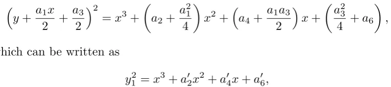
gen-eralized Weierstrass equation) is useful when working with fields of char-acteristic 2 and charchar-acteristic 3. If the charchar-acteristic of the field is not 2, then we can divide by 2 and complete the square:

y+ a1x

2 +

a3

2

2

=x3 +

a2+

a2₁ 4

x2+a4 +

a1a3

2

x+

a2₃ 4 +a6

,

which can be written as

y2₁ =x3+a′₂x2 +a′₄x+a′₆,

with y1 =y+a1x/2 +a3/2 and with some constants a′2, a′4, a′6. If the

charac-teristic is also not 3, then we can let x1 =x+a′2/3 and obtain

y₁2 =x3₁ +Ax1+B,

In most of this book, we will develop the theory using the Weierstrass equation, occasionally pointing out what modifications need to be made in characteristics 2 and 3. In Section 2.8, we discuss the case of characteristic 2 in more detail, since the formulas for the (nongeneralized) Weierstrass equation do not apply. In contrast, these formulas are correct in characteristic 3 for curves of the form y2 _{= x}3 _{+Ax+B, but there are curves that are not of}

this form. The general case for characteristic 3 can be obtained by using the present methods to treat curves of the form y2 _=x3_+Cx2_+Ax+B.

Finally, suppose we start with an equation

cy2 =dx3+ax+b

with c, d= 0. Multiply both sides of the equation by c3d2 to obtain (c2dy)2 = (cdx)3 + (ac2d)(cdx) + (bc3d2).

The change of variables

y1 =c2dy, x1 =cdx

yields an equation in Weierstrass form.

Later in this chapter, we will meet other types of equations that can be transformed into Weierstrass equations for elliptic curves. These will be useful in certain contexts.

For technical reasons, it is useful to add a point at infinity to an elliptic curve. In Section 2.3, this concept will be made rigorous. However, it is easiest to regard it as a point (_∞,_∞), usually denoted simply by _∞, sitting at the top of the y-axis. For computational purposes, it will be a formal symbol satisfying certain computational rules. For example, a line is said to pass through _∞ exactly when this line is vertical (i.e., x =constant). The point _∞ might seem a little unnatural, but we will see that including it has very useful consequences.

2.2 The Group Law

As we saw in Chapter 1, we could start with two points, or even one point, on an elliptic curve, and produce another point. We now examine this process in more detail.

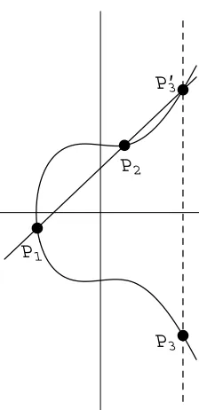
P1

P2

P3

P’3

Figure 2.2

Adding Points on an Elliptic Curve

Start with two points

P1 = (x1, y1), P2 = (x2, y2)

on an elliptic curve E given by the equation y2 _=x3_{+Ax+B. Define a new}

point P3 as follows. Draw the lineLthrough P1 and P2. We’ll see below that

L intersects E in a third point P₃′. Reflect P₃′ across the x-axis (i.e., change the sign of the y-coordinate) to obtain P3. We define

P1 +P2 =P3.

Examples below will show that this is not the same as adding coordinates of the points. It might be better to denote this operation by P1 +E P2, but we

opt for the simpler notation since we will never be adding points by adding coordinates.

Assume first that P1 = P2 and that neither point is ∞. Draw the line L

through P1 and P2. Its slope is

m= y2−y1 x2−x1

If x1 =x2, then L is vertical. We’ll treat this case later, so let’s assume that

x1 =x2. The equation of L is then

y =m(x₋x1) +y1.

To find the intersection with E, substitute to get

(m(x₋x1) +y1)2 =x3 +Ax+B.

This can be rearranged to the form

0 =x3 ₋m2x2 +_{· · ·} .

The three roots of this cubic correspond to the three points of intersection of L with E. Generally, solving a cubic is not easy, but in the present case we already know two of the roots, namely x1 and x2, since P1 and P2 are points

on both L and E. Therefore, we could factor the cubic to obtain the third value of x. But there is an easier way. As in Chapter 1, if we have a cubic polynomial x3 +ax2 +bx+c with roots r, s, t, then

x3 +ax2 +bx+c= (x₋r)(x₋s)(x₋t) = x3₋(r +s+t)x2 +_{· · ·} . Therefore,

r+s+t=₋a.

If we know two roots r, s, then we can recover the third as t=₋a₋r ₋s. In our case, we obtain

x=m2 ₋x1 −x2

and

y =m(x₋x1) +y1.

Now, reflect across the x-axis to obtain the pointP3 = (x3, y3):

x3 =m2−x1−x2, y3 =m(x1 −x3)−y1.

In the case thatx1 =x2 buty1 = y2, the line throughP1 andP2 is a vertical

line, which therefore intersects E in _∞. Reflecting _∞across the x-axis yields the same point _∞ (this is why we put _∞ at both the top and the bottom of the y-axis). Therefore, in this case P1+P2 =∞.

Now consider the case where P1 = P2 = (x1, y1). When two points on

a curve are very close to each other, the line through them approximates a tangent line. Therefore, when the two points coincide, we take the line L through them to be the tangent line. Implicit differentiation allows us to find the slope m of L:

2ydy dx = 3x

2 _{+A, so m=} dy

dx = 3x2

1 +A

2y1

Ify1 = 0 then the line is vertical and we setP1+P2 =∞, as before. (Technical

point:ify1 = 0, then the numerator 3x21+A = 0. See Exercise 2.5.) Therefore,

assume that y1 = 0. The equation of L is

y =m(x₋x1) +y1,

as before. We obtain the cubic equation

0 =x3 ₋m2x2 +_{· · ·} .

This time, we know only one root, namely x1, but it is a double root since L

is tangent to E at P1. Therefore, proceeding as before, we obtain

x3 =m2 −2x1, y3 =m(x1−x3)−y1.

Finally, suppose P2 = ∞. The line through P1 and ∞ is a vertical line

that intersects E in the point P₁′ that is the reflection of P1 across the x-axis.

When we reflect P′

1 across the x-axis to get P3 =P1 +P2, we are back at P1.

Therefore

P1 +∞=P1

for all points P1 on E. Of course, we extend this to include ∞+∞=∞.

Let’s summarize the above discussion:

GROUP LAW

LetE be an elliptic curve defined byy2 =x3+Ax+B. LetP1 = (x1, y1) and

P2 = (x2, y2) be points onE withP1, P2 = ∞. D efineP1+P2 =P3 = (x3, y3)

as follows:

1. Ifx1 =x2,then

x3 =m2 −x1 −x2, y3 =m(x1 −x3)−y1, wherem=

y2 −y1

x2 −x1

.

2. Ifx1 =x2 buty1 =y2,then P1+P2 =∞.

3. IfP1 =P2 andy1 = 0,then

x3 =m2 −2x1, y3 =m(x1−x3)−y1, wherem=

3x2₁ +A 2y1

.

4. IfP1 =P2 andy1 = 0,then P1 +P2 =∞.

M oreover,define

P +_∞=P

Note that whenP1 and P2 have coordinates in a fieldLthat containsAand

B, then P1 +P2 also has coordinates in L. Therefore E(L) is closed under

the above addition of points.

This addition of points might seem a little unnatural. Later (in Chapters 9 and 11), we’ll interpret it as corresponding to some very natural operations, but, for the present, let’s show that it has some nice properties.

THEOREM 2.1

T he addition ofpoints on an elliptic curveE satisfies the following properties: 1. (com m utativity)P1 +P2 =P2 +P1 for allP1, P2 on E.

2. (existence ofidentity)P +_∞=P for allpointsP on E.

3. (existence ofinverses)G ivenP onE,there existsP′ onE withP+P′ =

∞. T his pointP′ willusually be denoted₋P.

4. (associativity)(P1 +P2) +P3 =P1 + (P2+P3) for allP1, P2, P3 on E.

In other words,the points on E form an additive abelian group with_∞ as the identity elem ent.

PROOF The commutativity is obvious, either from the formulas or from the fact that the line through P1 and P2 is the same as the line through P2

and P1. The identity property of ∞ holds by definition. For inverses, let P′

be the reflection of P across the x-axis. Then P +P′ =_∞.

Finally, we need to prove associativity. This is by far the most subtle and nonobvious property of the addition of points on E. It is possible to define many laws of composition satisfying (1), (2), (3) for points onE, either simpler or more complicated than the one being considered. But it is very unlikely that such a law will be associative. In fact, it is rather surprising that the law of composition that we have defined is associative. After all, we start with two points P1 and P2 and perform a certain procedure to obtain a third

point P1 +P2. Then we repeat the procedure with P1 +P2 and P3 to obtain

(P1 +P2) +P3. If we instead start by adding P2 and P3, then computing

P1+ (P2+P3), there seems to be no obvious reason that this should give the

same point as the other computation.

The associative law can be verified by calculation with the formulas. There are several cases, depending on whether or not P1 =P2, and whether or not

P3 = (P1 +P2), etc., and this makes the proof rather messy. However, we

prefer a different approach, which we give in Section 2.4.

Warning: For the Weierstrass equation, ifP = (x, y), then ₋P = (x,₋y). For the generalized Weierstrass equation (2.1), this is no longer the case. If P = (x, y) is on the curve described by (2.1), then (see Exercise 2.9)

Example 2.1

The calculations of Chapter 1 can now be interpreted as adding points on elliptic curves. On the curve

y2 = x(x+ 1)(2x+ 1)

6 ,

we have

(0,0) + (1,1) = (1 2,−

1 2), (

1 2,−

1

2) + (1,1) = (24,−70). On the curve

y2 =x3 ₋25x, we have

2(₋4,6) = (₋4,6) + (₋4,6) =

1681 144 , −

62279 1728

.

We also have

(0,0) + (₋5,0) = (5,0), 2(0,0) = 2(₋5,0) = 2(5,0) =_∞.

The fact that the points on an elliptic curve form an abelian group is be-hind most of the interesting properties and applications. The question arises: what can we say about the groups of points that we obtain? Here are some examples.

1. An elliptic curve over a finite field has only finitely many points with coordinates in that finite field. Therefore, we obtain a finite abelian group in this case. Properties of such groups, and applications to cryp-tography, will be discussed in later chapters.

2. IfE is an elliptic curve defined overQ, thenE(Q) is a finitely generated abelian group. This is the Mordell-Weil theorem, which we prove in Chapter 8. Such a group is isomorphic to Zr ⊕F for some r _≥ 0 and some finite group F. The integer r is called the rank of E(Q). Determining r is fairly difficult in general. It is not known whether r can be arbitrarily large. At present, there are elliptic curves known with rank at least 28. The finite group F is easy to compute using the Lutz-Nagell theorem of Chapter 8. Moreover, a deep theorem of Mazur says that there are only finitely many possibilities forF, asE ranges over all elliptic curves defined over Q.

3. An elliptic curve over the complex numbers C is isomorphic to a torus. This will be proved in Chapter 9. The usual way to obtain a torus is as

Figure 2.3

An Elliptic Curve over C

4. If E is defined over R, then E(R) is isomorphic to the unit circle S1 or to S1 _⊕Z2. The first case corresponds to the case where the cubic

polynomial x3_{+Ax+B has only one real root (think of the ends of the}

graph in Figure 2.1(b) as being hitched together at the point_∞ to get a loop). The second case corresponds to the case where the cubic has three real roots. The closed loop in Figure 2.1(a) is the set S1_⊕{1_}, while the open-ended loop can be closed up using _∞ to obtain the set S1 _{⊕ {}0_}. If we have an elliptic curve E defined over R, then we can consider its complex points E(C). These form a torus, as in (3) above. The real points E(R) are obtained by intersecting the torus with a plane. If the plane passes through the hole in the middle, we obtain a curve as in Figure 2.1(a). If it does not pass through the hole, we obtain a curve as in Figure 2.1(b) (see Section 9.3).

If P is a point on an elliptic curve and k is a positive integer, then kP denotes P +P +_{· · ·}+P (with k summands). If k < 0, then kP = (₋P) + (₋P) +_{· · ·}(₋P), with_|k_| summands. To computekP for a large integer k, it is inefficient to add P to itself repeatedly. It is much faster to use successive doubling. For example, to compute 19P, we compute

2P, 4P = 2P+2P, 8P = 4P+4P, 16P = 8P+8P, 19P = 16P+2P+P.

This method allows us to computekP for very large k, say of several hundred digits, very quickly. The only difficulty is that the size of the coordinates of the points increases very rapidly if we are working over the rational numbers (see Theorem 8.18). However, when we are working over a finite field, for example Fp, this is not a problem because we can continually reduce mod p

law allows us to make these computations without worrying about what order we use to combine the summands.

The method of successive doubling can be stated in general as follows:

INTEGER TIMES A POINT

Letk be a positive integer and letP be a point on an elliptic curve. T he following procedure com puteskP.

1. Start witha =k, B =_∞, C =P.

2. Ifa is even,leta=a/2,and letB =B, C = 2C.

3. Ifa is odd,leta=a₋1,and letB =B+C, C =C.

4. Ifa= 0,go to step 2.

5. O utputB.

T he outputB iskP (see Exercise 2.8).

On the other hand, if we are working over a large finite field and are given points P and kP, it is very difficult to determine the value ofk. This is called the discrete logarithm problem for elliptic curves and is the basis for the cryptographic applications that will be discussed in Chapter 6.

2.3 Projective Space and the Point at Infinity

We all know that parallel lines meet at infinity. Projective space allows us to make sense out of this statement and also to interpret the point at infinity on an elliptic curve.

LetKbe a field. Two-dimensionalprojective space P2_K overK is given by equivalence classes of triples (x, y, z) withx, y, z _∈K and at least one ofx, y, z nonzero. Two triples (x1, y1, z1) and (x2, y2, z2) are said to be equivalent if

there exists a nonzero element λ_∈K such that

(x1, y1, z1) = (λx2, λy2, λz2).

We write (x1, y1, z1) ∼ (x2, y2, z2). The equivalence class of a triple only

depends on the ratios of x to y to z. Therefore, the equivalence class of (x, y, z) is denoted (x: y :z).

If (x : y : z) is a point with z = 0, then (x: y : z) = (x/z : y/z : 1). These are the “finite” points in P2

K. However, if z = 0 then dividing by z should

be thought of as giving _∞ in either the x or y coordinate, and therefore the points (x : y : 0) are called the “points at infinity” in P2

infinity on an elliptic curve will soon be identified with one of these points at infinity in P2_K.

The two-dimensional affine plane over K is often denoted

A2_K =_{(x, y)_∈K _×K_}. We have an inclusion

A2_K ֒_→P2_K

given by

(x, y)_→(x: y : 1).

In this way, the affine plane is identified with the finite points in P2

K. Adding

the points at infinity to obtainP2_K can be viewed as a way of “compactifying” the plane (see Exercise 2.10).

A polynomial is homogeneous of degree n if it is a sum of terms of the form axi_yj_zk _{with a ∈ K and i +j +k = n. For example, F(x, y, z) =}

2x3₋5xyz+ 7yz2 is homogeneous of degree 3. If a polynomial F is homoge-neous of degree n then F(λx, λy, λz) = λnF(x, y, z) for all λ_∈ K. It follows that if F is homogeneous of some degree, and (x1, y1, z1) ∼(x2, y2, z2), then

F(x1, y1, z1) = 0 if and only ifF(x2, y2, z2) = 0. Therefore, a zero of F inP2K

does not depend on the choice of representative for the equivalence class, so the set of zeros of F in P2_K is well defined.

IfF(x, y, z) is an arbitrary polynomial in x, y, z, then we cannot talk about a point in P2_K where F(x, y, z) = 0 since this depends on the representative (x, y, z) of the equivalence class. For example, let F(x, y, z) = x2 _{+ 2y−3z.}

Then F(1,1,1) = 0, so we might be tempted to say that F vanishes at (1 : 1 : 1). But F(2,2,2) = 2 and (1 : 1 : 1) = (2 : 2 : 2). To avoid this problem, we need to work with homogeneous polynomials.

If f(x, y) is a polynomial in x and y, then we can make it homogeneous by inserting appropriate powers of z. For example, iff(x, y) =y2₋x3₋Ax₋B, then we obtain the homogeneous polynomial F(x, y, z) = y2z₋x3 ₋Axz2 ₋ Bz3_{. If F is homogeneous of degree n then}

F(x, y, z) =znf(x z,

y z)

and

f(x, y) = F(x, y,1).

We can now see what it means for two parallel lines to meet at infinity. Let

y =mx+b1, y =mx+b2

be two nonvertical parallel lines with b1 = b2. They have the homogeneous

forms

(The preceding discussion considered only equations of the form f(x, y) = 0 and F(x, y, z) = 0; however, there is nothing wrong with rearranging these equations to the form “homogeneous of degree n = homogeneous of degree n.”) When we solve the simultaneous equations to find their intersection, we obtain

z = 0 and y =mx.

Since we cannot have all of x, y, z being 0, we must have x= 0. Therefore, we can rescale by dividing by x and find that the intersection of the two lines is

(x: mx: 0) = (1 :m: 0).

Similarly, if x = c1 and x = c2 are two vertical lines, they intersect in the

point (0 : 1 : 0). This is one of the points at infinity in P2_K.

Now let’s look at the elliptic curve E given by y2 _{= x}3 _{+ Ax+ B. Its}

homogeneous form is y2z = x3 + Axz2 + Bz3. The points (x, y) on the original curve correspond to the points (x: y : 1) in the projective version. To see what points on E lie at infinity, set z = 0 and obtain 0 = x3. Therefore x= 0, andy can be any nonzero number (recall that (0 : 0 : 0) is not allowed). Rescale by y to find that (0 :y : 0) = (0 : 1 : 0) is the only point at infinity on E. As we saw above, (0 : 1 : 0) lies on every vertical line, so every vertical line intersects E at this point at infinity. Moreover, since (0 : 1 : 0) = (0 :₋1 : 0), the “top” and the “bottom” of the y-axis are the same.

There are situations where using projective coordinates speeds up compu-tations on elliptic curves (see Section 2.6). However, in this book we almost always work in affine (nonprojective) coordinates and treat the point at infin-ity as a special case when needed. An exception is the proof of associativinfin-ity of the group law given in Section 2.4, where it will be convenient to have the point at infinity treated like any other point (x:y : z).

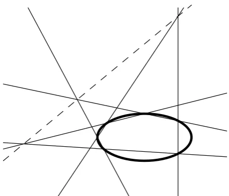
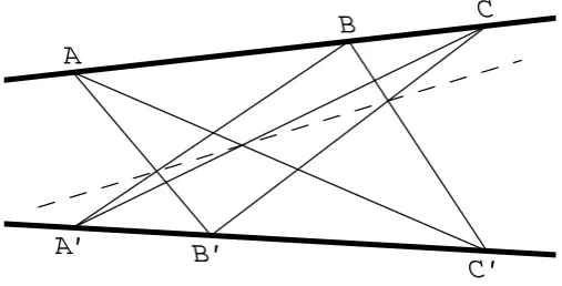
2.4 Proof of Associativity

In this section, we prove the associativity of addition of points on an elliptic curve. The reader who is willing to believe this result may skip this section without missing anything that is needed in the rest of the book. However, as corollaries of the proof, we will obtain two results, namely the theorems of Pappus and Pascal, that are not about elliptic curves but which are interesting in their own right.

The basic idea is the following. Start with an elliptic curve E and points P, Q, R on E. To compute ₋((P +Q) +R) we need to form the lines ℓ1 =

P Q, m2 = ∞, P +Q, and ℓ3 = R, P +Q, and see where they intersect E.

To compute ₋((P + (Q+R)) we need to form the lines m1 = QR, ℓ2 =

lie on E, except possibly for P33. We show in Theorem 2.6 that having the

eight points Pij = P33 on E forces P33 to be on E. Since ℓ3 intersects E at

the points R, P +Q,₋((P +Q) +R), we must have ₋((P +Q) +R) =P33.

Similarly, ₋(P + (Q+R)) =P33, so

−((P +Q) +R) = ₋(P + (Q+R)),

which implies the desired associativity.

There are three main technicalities that must be treated. First, some of the points Pij could be at infinity, so we need to use projective coordinates.

Second, a line could be tangent to E, which means that two Pij could be

equal. Therefore, we need a careful definition of the order to which a line intersects a curve. Third, two of the lines could be equal. Dealing with these technicalities takes up most of our attention during the proof.

First, we need to discuss lines in P2_K. The standard way to describe a line is by a linear equation: ax+by +cz = 0. Sometimes it is useful to give a parametric description:

x=a1u+b1v

y =a2u+b2v (2.2)

z =a3u+b3v

where u, v run through K, and at least one ofu, v is nonzero. For example, if a= 0, the line

ax+by+cz = 0

can be described by

x=₋(b/a)u₋(c/a)v, y =u, z =v.

Suppose all the vectors (ai, bi) are multiples of each other, say (ai, bi) =

λi(a1, b1). Then (x, y, z) = x(1, λ2, λ3) for all u, v such that x= 0. So we get

a point, rather than a line, in projective space. Therefore, we need a condition on the coefficients a1, . . . , b3 that ensure that we actually get a line. It is not

hard to see that we must require the matrix

⎛ ⎝aa12 bb12

a3 b3

⎞ ⎠

to have rank 2 (cf. Exercise 2.12).

If (u1, v1) = λ(u2, v2) for some λ ∈ K×, then (u1, v1) and (u2, v2) yield

equivalent triples (x, y, z). Therefore, we can regard (u, v) as running through points (u : v) in 1-dimensional projective space P1

K. Consequently, a line

We need to quantify the order to which a line intersects a curve at a point. The following gets us started.

LEMMA 2.2

LetG(u, v) be a nonzero hom ogeneous polynom ialand let(u0 : v0) ∈ P1K.

T hen there exists an integerk_≥0 and a polynom ialH(u, v) withH(u0, v0) =

0 such that

G(u, v) = (v0u−u0v)kH(u, v).

PROOF Suppose v0 = 0. Let m be the degree of G. Let g(u) = G(u, v0).

By factoring out as large a power of u₋u0 as possible, we can write g(u) =

(u₋u0)kh(u) for some k and for some polynomial h of degree m−k with

h(u0) = 0. Let H(u, v) = (vm−k/v0m)h(uv0/v), so H(u, v) is homogeneous of

degree m₋k. Then

G(u, v) =

v v0

m

guv0 v

= v

m−k

vm

0

(v0u−u0v)kh

_uv0

v

=(v0u−u0v)kH(u, v),

as desired.

If v0 = 0, then u0 = 0. Reversing the roles of u and v yields the proof in

this case.

Let f(x, y) = 0 (where f is a polynomial) describe a curve C in the affine plane and let

x=a1t+b1, y=a2t+b2

be a line L written in terms of the parameter t. Let ˜

f(t) = f(a1t+b1, a2t+b2).

Then L intersects C when t = t0 if ˜f(t0) = 0. If (t − t0)2 divides ˜f(t),

then L is tangent to C (if the point corresponding to t0 is nonsingular. See

Lemma 2.5). More generally, we say that L intersects C to order n at the point (x, y) corresponding to t=t0 if (t−t0)n is the highest power of (t−t0)

that divides ˜f(t).

The homogeneous version of the above is the following. Let F(x, y, z) be a homogeneous polynomial, so F = 0 describes a curve C in P2_K. Let L be a line given parametrically by (2.2) and let

˜

F(u, v) =F(a1u+b1v, a2u+b2v, a3u+b3v).

We say that L intersects C to order n at the point P = (x0 : y0 : z0)

corresponding to (u : v) = (u0 : v0) if (v0u−u0v)n is the highest power of

(v0u−u0v) dividing ˜F(u, v). We denote this by

If ˜F is identically 0, then we let ordL,P(F) = ∞. It is not hard to show that

ordL,P(F) is independent of the choice of parameterization of the lineL. Note

thatv =v0 = 1 corresponds to the nonhomogeneous situation above, and the

definitions coincide (at least when z = 0). The advantage of the homogeneous formulation is that it allows us to treat the points at infinity along with the finite points in a uniform manner.

LEMMA 2.3

LetL1 and L2 be lines intersecting in a pointP, and, for i = 1,2, let

Li(x, y, z) be a linear polynom ialdefiningLi. T hen ordL1,P(L2) = 1 unless

L1(x, y, z) = αL2(x, y, z) for som e constantα, in which caseordL1,P(L2) =

∞.

PROOF When we substitute the parameterization for L1 into L2(x, y, z),

we obtain ˜L2, which is a linear expression in u, v. Let P correspond to (u0 :

v0). Since ˜L2(u0, v0) = 0, it follows that ˜L2(u, v) = β(v0u−u0v) for some

constant β. If β = 0, then ordL1,P(L2) = 1. If β = 0, then all points on

L1 lie on L2. Since two points in P2K determine a line, and L1 has at least

three points (P1

K always contains the points (1 : 0),(0 : 1),(1 : 1)), it follows

that L1 and L2 are the same line. Therefore L1(x, y, z) is proportional to

L2(x, y, z).

Usually, a line that intersects a curve to order at least 2 is tangent to the curve. However, consider the curve C defined by

F(x, y, z) =y2z₋x3 = 0. Let

x=au, y =bu, z =v

be a line through the point P = (0 : 0 : 1). Note that P corresponds to (u : v) = (0 : 1). We have ˜F(u, v) = u2_(b2_{v −a}3_{u), so every line through P}

intersects C to order at least 2. The line with b = 0, which is the best choice for the tangent atP, intersectsC to order 3. The affine part ofC is the curve y2 = x3, which is pictured in Figure 2.7. The point (0,0) is a singularity of the curve, which is why the intersections at P have higher orders than might be expected. This is a situation we usually want to avoid.

DEFINITION 2.4 A curveC inP2_K defined byF(x, y, z) = 0 is said to be

nonsingular at a pointP ifat least one ofthe partialderivativesFx, Fy, Fz

is nonzero atP.

We have

Fx =−3x2 −Az2, Fy = 2yz, Fz =y2 −2Axz−3Bz2.

Suppose P = (x : y : z) is a singular point. If z = 0, then Fx = 0 implies

x = 0 and Fz = 0 implies y = 0, so P = (0 : 0 : 0), which is impossible.

Therefore z = 0, so we may take z = 1 (and therefore ignore it). If Fy = 0,

theny = 0. Since (x:y : 1) lies on the curve, xmust satisfy x3+Ax+B = 0. If Fx = −(3x2 +A) = 0, then x is a root of a polynomial and a root of its

derivative, hence a double root. Since we assumed that the cubic polynomial has no multiple roots, we have a contradiction. Therefore an elliptic curve has no singular points. Note that this is true even if we are considering points with coordinates in K (= algebraic closure of K). In general, by a nonsingular curve we mean a curve with no singular points inK.

If we allow the cubic polynomial to have a multiple rootx, then it is easy to see that the curve has a singularity at (x : 0 : 1). This case will be discussed in Section 2.10.

If P is a nonsingular point of a curve F(x, y, z) = 0, then the tangent line at P is

Fx(P)x+Fy(P)y+Fz(P)z = 0.

For example, if F(x, y, z) = y2z₋x3 ₋Axz2 ₋Bz3 = 0, then the tangent line at (x0 : y0 : z0) is

(₋3x2_{0 −}Az₀2)x+ 2y0z0y+ (y02 −2Ax0z0 −3Bz02)z = 0.

If we set z0 =z = 1, then we obtain

(₋3x2_{0 −}A)x+ 2y0y+ (y02 −2Ax0−3B) = 0.

Using the fact that y20 =x30+Ax0+B, we can rewrite this as

(₋3x2₀₋A)(x₋x0) + 2y0(y−y0) = 0.

This is the tangent line in affine coordinates that we used in obtaining the formulas for adding a point to itself on an elliptic curve. Now let’s look at the point at infinity on this curve. We have (x0 : y0 : z0) = (0 : 1 : 0). The

tangent line is given by 0x+ 0y+z = 0, which is the “line at infinity” inP2_K. It intersects the elliptic curve only in the point (0 : 1 : 0). This corresponds to the fact that _∞+_∞=_∞ on an elliptic curve.

LEMMA 2.5

LetF(x, y, z) = 0 define a curveC. IfP is a nonsingular point ofC, then there is exactly one line in P2_K that intersectsC to order at least 2,and it is the tangent toC atP.

to P. Then ˜F = (v0u−u0v)kH(u, v) for some H(u, v) with H(u0, v0) = 0.

Therefore,

˜

Fu(u, v) =kv0(v0u−u0v)k−1H(u, v) + (v0u−u0v)kHu(u, v)

and

˜

Fv(u, v) = −ku0(v0u−u0v)k−1H(u, v) + (v0u−u0v)kHv(u, v).

It follows that k _≥2 if and only if ˜Fu(u0, v0) = ˜Fv(u0, v0) = 0.

Suppose k_≥2. The chain rule yields ˜

Fu =a1Fx+a2Fy+a3Fz = 0, F˜v =b1Fx+b2Fy +b3Fz = 0 (2.3)

at P. Recall that since the parameterization (2.2) yields a line, the vectors (a1, a2, a3) and (b1, b2, b3) must be linearly independent.

Suppose L′ is another line that intersects C to order at least 2. Then we obtain another set of equations

a′₁Fx+a′2Fy+a′3Fz = 0, b′1Fx+b′2Fy +b′3Fz = 0

at P.

If the vectors a′ = (a′₁, a′₂, a′₃) and b′ = (b′₁, b′₂, b′₃) span the same plane in K3 as a= (a1, a2, a3) and b = (b1, b2, b3), then

a′ =αa+βb, b′ =γa+δb

for some invertible matrix

α β γ δ

. Therefore,

ua′ +vb′ = (uα+vγ)a+ (uβ+vδ)b =u1a+v1b

for a new choice of parameters u1, v1. This means thatL and L′ are the same

line.

If L and L′ _{are different lines, then a,b and a}′_,b′ _{span different planes, so} the vectors a,b,a′,b′ must span all ofK3. Since (Fx, Fy, Fz) has dot product

0 with these vectors, it must be the 0 vector. This means that P is a singular point, contrary to our assumption.

Finally, we need to show that the tangent line intersects the curve to order at least 2. Suppose, for example, that Fx = 0 at P. The cases where Fy = 0

and Fz = 0 are similar. The tangent line can be given the parameterization

x=₋(Fy/Fx)u−(Fz/Fx)v, y =u, z =v,

so

a1 =−Fy/Fx, b1 =−Fz/Fx, a2 = 1, b2 = 0, a3 = 0, b3 = 1

in the notation of (2.2). Substitute into (2.3) to obtain

˜

By the discussion at the beginning of the proof, this means that the tangent line intersects the curve to order k _≥2.

The associativity of elliptic curve addition will follow easily from the next result. The proof can be simplified if the pointsPij are assumed to be distinct.

The cases where points are equal correspond to situations where tangent lines are used in the definition of the group law. Correspondingly, this is where it is more difficult to verify the associativity by direct calculation with the formulas for the group law.

THEOREM 2.6

LetC(x, y, z) be a hom ogeneous cubic polynom ial,and letC be the curve in

P2_K described byC(x, y, z) = 0. Letℓ1, ℓ2, ℓ3 and m1, m2, m3 be lines in P2K

such thatℓi = mj for alli, j. LetPij be the point of intersection ofℓi and

mj. SupposePij is a nonsingular point on the curveC for all(i, j) = (3,3).

In addition, we require that if, for som e i, there are k _≥ 2 of the points

Pi1, Pi2, Pi3 equalto the sam e point, then ℓi intersectsC to order at leastk

at this point. A lso, if, for som ej, there arek _≥ 2 of the pointsP1j, P2j, P3j

equalto the sam e point,then mj intersectsC to order atleastk atthis point.

T hen P33 also lies on the curveC.

PROOF Expressℓ1 in the parametric form (2.2). ThenC(x, y, z) becomes

˜

C(u, v). The line ℓ1 passes through P11, P12, P13. Let (u1 : v1),(u2 :v2),(u3 :

v3) be the parameters on ℓ1 for these points. Since these points lie on C, we

have ˜C(ui, vi) = 0 for i = 1,2,3.

Let mj have equation mj(x, y, z) = ajx+ bjy +cjz = 0. Substituting

the parameterization for ℓ1 yields ˜mj(u, v). Since Pij lies on mj, we have

˜

mj(uj, vj) = 0 forj = 1,2,3. Sinceℓ1 =mj and since the zeros of ˜mj yield the

intersections of ℓ1 and mj, the function ˜mj(u, v) vanishes only at P1j, so the

linear form ˜mj is nonzero. Therefore, the product ˜m1(u, v) ˜m2(u, v) ˜m3(u, v)

is a nonzero cubic homogeneous polynomial. We need to relate this product to ˜C.

LEMMA 2.7

LetR(u, v) andS(u, v) be hom ogeneous polynom ials ofdegree 3,withS(u, v)

not identically 0, and suppose there are three points(ui : vi),i = 1,2,3, at

which R and S vanish. M oreover, ifk of these points are equalto the sam e point, we require thatR and S vanish to order at leastk at this point (that is,(viu−uiv)k dividesR and S). T hen there is a constantα ∈K such that

R =αS.

PROOF First, observe that a nonzero cubic homogeneous polynomial S(u, v) can have at most 3 zeros (u : v) in P1

This can be proved as follows. Factor off the highest possible power of v, say vk. Then S(u, v) vanishes to order k at (1 : 0), and S(u, v) =vkS0(u, v) with

S0(1,0) = 0. Since S0(u,1) is a polynomial of degree 3−k, the polynomial

S0(u,1) can have at most 3−k zeros, counting multiplicities (it has exactly

3₋k if K is algebraically closed). All points (u: v) = (1 : 0) can be written in the form (u: 1), so S0(u, v) has at most 3−k zeros. Therefore,S(u, v) has

at most k+ (3₋k) = 3 zeros in P1_K.

It follows easily that the condition that S(u, v) vanish to order at least k could be replaced by the condition that S(u, v) vanish to order exactly k. However, it is easier to check “at least” than “exactly.” Since we are allowing the possibility that R(u, v) is identically 0, this remark does not apply to R.

Let (u0,: v0) be any point inP1K not equal to any of the (ui :vi). (Technical

point: If K has only two elements, then P1_K has only three elements. In this case, enlarge K to GF(4). Theα we obtain is forced to be inK since it is the ratio of a coefficient ofR and a coefficient ofS, both of which are inK.) Since S can have at most three zeros, S(u0, v0) = 0. Let α = R(u0, v0)/S(u0, v0).

Then R(u, v)₋αS(u, v) is a cubic homogeneous polynomial that vanishes at the four points (ui : vi), i = 0,1,2,3. Therefore R−αS must be identically

zero.

Returning to the proof of the theorem, we note that ˜C and ˜m1m˜2m˜3 vanish

at the points (ui : vi), i = 1,2,3. Moreover, if k of the points P1j are the

same point, then k of the linear functions vanish at this point, so the product ˜

m1(u, v) ˜m2(u, v) ˜m3(u, v) vanishes to order at least k. By assumption, ˜C

vanishes to order at least k in this situation. By the lemma, there exists a constant α such that

˜

C =αm˜1m˜2m˜3.

Let

C1(x, y, z) =C(x, y, z)−αm1(x, y, z)m2(x, y, z)m3(x, y, z).

The lineℓ1 can be described by a linear equationℓ1(x, y, z) = ax+by+cz =

0. At least one coefficient is nonzero, so let’s assume a = 0. The other cases are similar. The parameterization of the line ℓ1 can be taken to be

x=₋(b/a)u₋(c/a)v, y =u, z =v. (2.4)

Then ˜C1(u, v) = C1(−(b/a)u−(c/a)v, u, v). WriteC1(x, y, z) as a polynomial

in x with polynomials in y, z as coefficients. Writing

xn = (1/an) ((ax+by+cz)₋(by+cz))n = (1/an) ((ax+by+cz)n +_{· · ·}),

we can rearrange C1(x, y, z) to be a polynomial in ax+by +cz whose

coeffi-cients are polynomials in y, z:

Substituting (2.4) into (2.5) yields

0 = ˜C1(u, v) =a0(u, v),

sinceax+by+cz vanishes identically whenx, y, z are written in terms ofu, v. Thereforea0(y, z) =a0(u, v) is the zero polynomial. It follows from (2.5) that

C1(x, y, z) is a multiple of ℓ1(x, y, z) = ax+by +cz.

Similarly, there exists a constant β such that C(x, y, z)₋βℓ1ℓ2ℓ3 is a

mul-tiple of m1.

Let

D(x, y, z) =C ₋αm1m2m3−βℓ1ℓ2ℓ3.

Then D(x, y, z) is a multiple of ℓ1 and a multiple of m1.

LEMMA 2.8

D(x, y, z) is a m ultiple ofℓ1(x, y, z)m1(x, y, z).

PROOF Write D = m1D1. We need to show that ℓ1 divides D1. We

could quote some result about unique factorization, but instead we proceed as follows. Parameterize the line ℓ1 via (2.4) (again, we are considering the

case a= 0). Substituting this into the relationD=m1D1 yields ˜D= ˜m1D˜1.

Sinceℓ1 dividesD, we have ˜D= 0. Sincem1 =ℓ1, we have ˜m1 = 0. Therefore

˜

D1(u, v) is the zero polynomial. As above, this implies that D1(x, y, z) is a

multiple of ℓ1, as desired.

By the lemma,

D(x, y, z) = ℓ1m1ℓ,

where ℓ(x, y, z) is linear. By assumption, C = 0 at P22, P23, P32. Also, ℓ1ℓ2ℓ3

and m1m2m3 vanish at these points. Therefore, D(x, y, z) vanishes at these

points. Our goal is to show that D is identically 0.

LEMMA 2.9

ℓ(P22) =ℓ(P23) =ℓ(P32) = 0.

PROOF First suppose that P13 = P23. If ℓ1(P23) = 0, then P23 is on

the line ℓ1 and also on ℓ2 and m3 by definition. Therefore, P23 equals the

intersectionP13 ofℓ1 and m3. Since P23 and P13 are for the moment assumed

to be distinct, this is a contradiction. Therefore ℓ1(P23)= 0. Since D(P23) =

0, it follows that m1(P23)ℓ(P23) = 0.

Suppose now that P13 = P23. Then, by the assumption in the

theo-rem, m3 is tangent to C at P23, so ordm3,P23(C) ≥ 2. Since P13 = P23

and P23 lies on m3, we have ordm3,P23(ℓ1) = ordm3,P23(ℓ2) = 1.

ordm3,P23(D) ≥2, since D is a sum of terms, each of which vanishes to order

at least 2. But ordm3,P23(ℓ1) = 1, so we have

ordm3,P23(m1ℓ) = ordm3,P23(D)−ordm3,P23(ℓ1)≥1.

Therefore m1(P23)ℓ(P23) = 0.

In both cases, we have m1(P23)ℓ(P23) = 0.

If m1(P23) = 0, then ℓ(P23) = 0, as desired.

If m1(P23) = 0, then P23 lies on m1, and also on ℓ2 and m3, by definition.

Therefore, P23 = P21, since ℓ2 and m1 intersect in a unique point. By

as-sumption, ℓ2 is therefore tangent to C at P23. Therefore, ordℓ2,P23(C) ≥ 2.

As above, ordℓ2,P23(D)≥2, so

ordℓ2,P23(ℓ1ℓ) ≥1.

If in this case we have ℓ1(P23) = 0, then P23 lies on ℓ1, ℓ2, m3. Therefore

P13 =P23. By assumption, the line m3 is tangent to C at P23. Since P23 is a

nonsingular point ofC, Lemma 2.5 says thatℓ2 =m3, contrary to hypothesis.

Therefore, ℓ1(P23) = 0, so ℓ(P23) = 0.

Similarly, ℓ(P22) =ℓ(P32) = 0.

If ℓ(x, y, z) is identically 0, then D is identically 0. Therefore, assume that ℓ(x, y, z) is not zero and hence it defines a line ℓ.

First suppose thatP23, P22, P32 are distinct. Thenℓandℓ2 are lines through

P23 and P22. Therefore ℓ = ℓ2. Similarly, ℓ = m2. Therefore ℓ2 = m2,

contradiction.

Now suppose that P32 =P22. Then m2 is tangent to C at P22. As before,

ordm2,P22(ℓ1m1ℓ) ≥2.

We want to show that this forces ℓ to be the same line as m2.

If m1(P22) = 0, then P22 lies on m1, m2, ℓ2. Therefore, P21 = P22. This

means that ℓ2 is tangent toC atP22. By Lemma 2.5, ℓ2 =m2, contradiction.

Therefore, m1(P22) = 0.

Ifℓ1(P22)= 0, then ordm2,P22(ℓ)≥2. This means that ℓis the same line as

m2.

If ℓ1(P22) = 0, then P22 = P32 lies on ℓ1, ℓ2, ℓ3, m2, so P12 = P22 =

P32. Therefo