Computer Animation

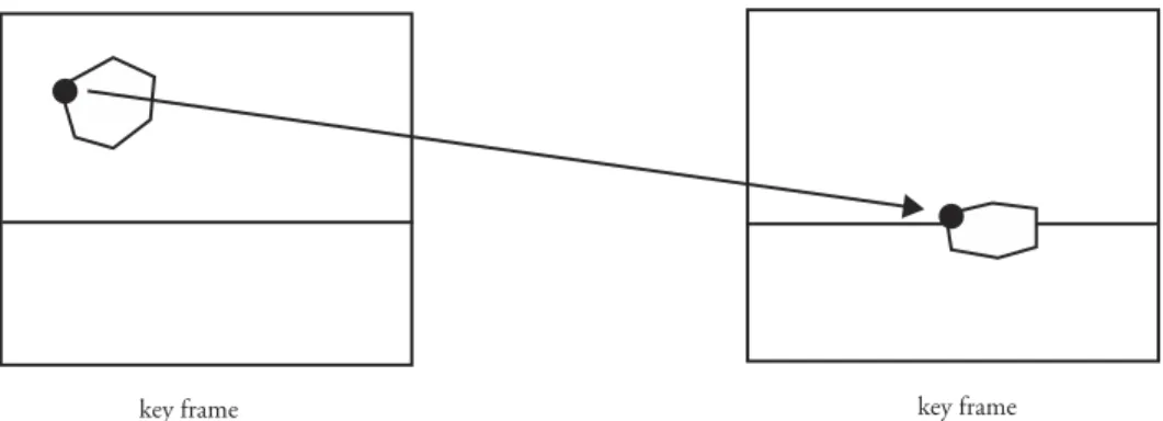
Just as we at the National Research Council of Canada were fortunate to work with artists and animators in the early days of computer animation development. In the late 1960s and 1970s, he collaborated with Nestor Burtnyk, who wrote the original keyframe interpolation software that became the basis of the first computer animation system.

Preface

Overview

Motion control methods can also be discussed in terms of the level of abstraction at which the animator works. A high level of abstraction frees the animator from dealing with the countless details required to produce a piece of animation.

Organization of the Book

In practice, the collection of techniques and algorithms used in computer animation forms a continuum from low to high levels of abstraction. High-level algorithms, on the other hand, require less specific information from the animator and more computation.

Acknowledgments

Appendix A presents rendering issues often involved in producing images for computer animation: double buffering, compositing, computer motion blur, and shadows. It assumes knowledge of the use of framebuffers, of how a z-buffer display algorithm works, and of aliasing issues.

For many people, computer animation is synonymous with big screen events such as Star Wars, Toy Story and Titanic. This book does not address the issues related to a specific venue, but it does present the algorithms and techniques used to do animation in all of them.

Introduction

Perception

Recently in the literature, it has been argued that gaze persistence is not the mechanism responsible for successful viewing of film and video as continuous images. One is the frame rate, the number of images per second displayed in the viewing process.

The Heritage of Animation

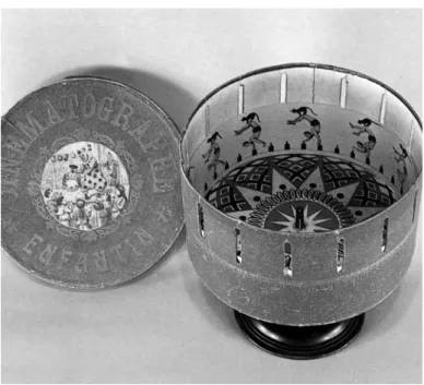
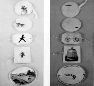
• Early Devices
• The Early Days of “Conventional” Animation
• Disney
• Contributions of Others
• Other Media for Animation
• Principles of Computer Animation

Each of the planes can move in six directions (right, left, up, down, in, out), and the camera can zoom in and out (see Figure 1.4). Many important animators at these studios were graduates of Disney or Bray studios.

Figure 1.1 A thaumatrope

Animation Production

• Computer Animation Production Tasks
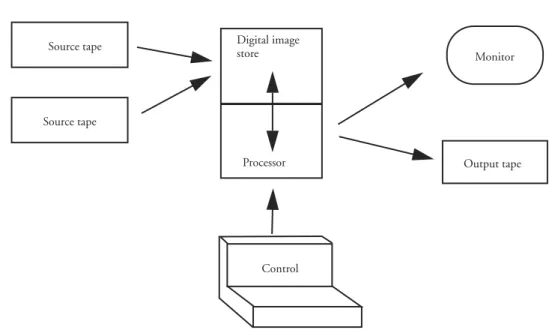
• Digital Editing
• Digital Video

A compromise between speed and quality can be made at any of the three stages of creating a computer animation frame: model building, motion control, and rendering. First, desktop animation has become cheap enough to be within reach of consumers.

Figure 1.9 Simplified example of a time line used for nonlinear digital editing

A Brief History of Computer Animation

• Early Activity
• The Middle Years

One of the earliest uses of computer graphics in film was the modeling and animation of spaceships. PDI used computer graphics to create large crowds in mid-1980s Bud Bowl commercials.

Chapter Summary

Laybourne, The Animation Book: A Complete Guide to Animated Filmmaking—from Flip-Books to Sound Cartoons to 3-D Animation, Three Rivers Press, New York, 1998. Thomas, Disneyjeva umetnost animacije od Mickeyja Mousea do »Lepotice in zveri« ,” Hyperion, New York, 1991.

Spaces and Transformations

The first serves as a quick review of the basics of the computer graphics display pipeline and discusses round-off error control when repeatedly transforming data. It is assumed that the reader has already been exposed to transformation matrices, homogeneous coordinates and the display pipeline, including the perspective transformation;.

Technical Background

The Display Pipeline

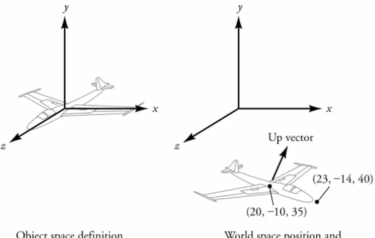
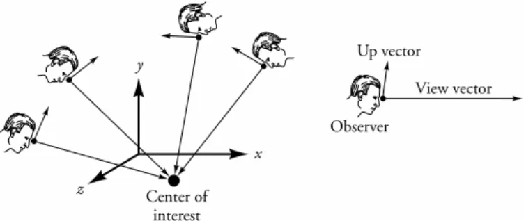
The parameters of the observer include its position and orientation, consisting of the gaze direction and the upward vector. The difference between a user-supplied up direction vector and an up vector is that the up vector is by definition perpendicular to the view direction vector.

Figure 2.1 Demonstrating the up vector flip as observer’s position passes straight over center of interest

Homogeneous Coordinates and the Transformation Matrix

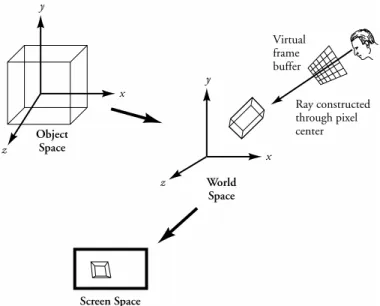
If the rays are constructed in world space based on pixel coordinates of a virtual frame buffer positioned in front of the observer, then the progression through spaces for ray casting reduces to the transformations shown in Figure 2.4. In the case of the transformations rotation, translation and non-zero scaling, the matrix always has a computable inverse.

Figure 2.4 Transformation through spaces using ray casting

Compounding Transformations

The 4x4 transformation matrix used in one of the notations is the transpose of the 4x4 transformation matrix used in the other notation.

Multiplying Transformation Matrices

Basic Transformations

A nonuniform scale allows independent scale factors to be applied to the x-, y-, and z-coordinates of a point and is formed by placing Sx, Sy, and Sz along the diagonal, as shown in Equation 2.10. A uniform scale can also be represented by setting the lowest rightmost value to 1/S, as in Equation 2.11.

Representing an Arbitrary Orientation

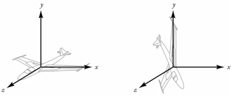
Assuming no longitudinal rotation (roll), the desired X-axis can be formed by taking the cross product of the original y-axis and the desired Z-axis. The desired Y-axis can then be formed by taking the cross product of the desired Z-axis and the desired X-axis.

Figure 2.6 Projection of desired orientation vector onto y -z plane

Extracting Transformations from a Matrix

In the example of transforming the plane, the desired Z-axis is the desired orientation vector. If the composite transformation matrix contains a uniform scale factor, then the rows of the 3x3 submatrix form orthogonal vectors of uniform length.

Description of Transformations in the Display Pipeline

Perspective matrix multiplication The perspective matrix multiplication is the first part of the perspective transformation. These intervals are arbitrary and can be set to anything by appropriately forming the perspective matrix. Perspective division Each point produced by the perspective matrix multiplication has a non-unit fourth component representing the perspective division by z.

Round-off Error Considerations

In the case of the moon, the transformation matrix is ​​initialized with the x-axis translation matrix. Take the cross product of the third row (column) and the first row (column), normalize it and place it in the second row (column). The error has just been moved so that the matrix columns are orthonormal and the error may be less noticeable.

Figure 2.10 Rotation by applying incremental rotation matrices to points

Orientation Representation

• Fixed Angle Representation
• Euler Angle Representation
• Angle and Axis
• Quaternions

A slight change to the third parameter will slightly rotate the object around the global z-axis, since this is the rotation applied last to the data points. However, as explained above, the object can no longer directly rotate about the x-axis from the first key orientation due to the 90-degree rotation of the y-axis. The rotation of the x-axis, represented by the transformation matrix Rx(α), is followed by the rotation of the y-axis, represented by the transformation matrix Ry(β), about the y-axis of the local, rotated coordinate system.

Figure 2.15 Fixed angle representation

Chapter Summary

Procedures and algorithms are indeed used, but in a very direct way where the animator has very specific expectations about the movement that will be produced on a frame-by-frame basis. Chapter 4, on advanced algorithms, addresses more sophisticated techniques, in which the animator sacrifices some precision to produce motion with certain desired characteristics. The high-level algorithms of the next chapter leave some uncertainty about how the objects will be positioned for any particular frame.

Interpolation

There is little uncertainty about the positions and orientations to be produced, and the computer is only used to calculate the actual values.

Interpolation and Basic Techniques

The Appropriate Function

In the latter case, a rough line can be used as the animator quickly gets a feel for how repositioning the control points affects the shape of the curve. Functions that approximate some or all of the control information include Bezier curves and B-splines. Mathematically, smoothness is determined by how many of the derivatives of the curve equation are continuous.

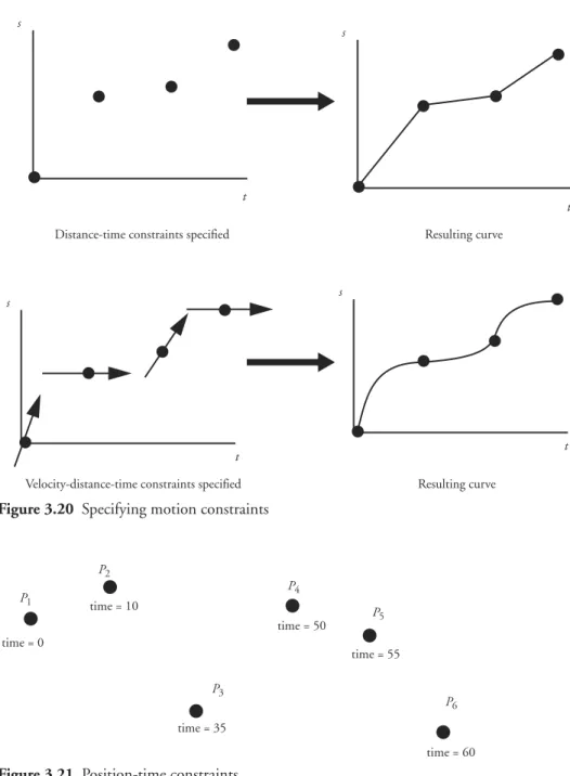
Controlling the Motion Along a Curve

• Computing Arc Length
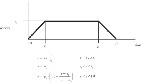
• Speed Control
• Ease-in/Ease-out
• Constant Acceleration: Parabolic Ease-In/Ease-Out
• General Distance-Time Functions
• Curve Fitting to Position-Time Pairs

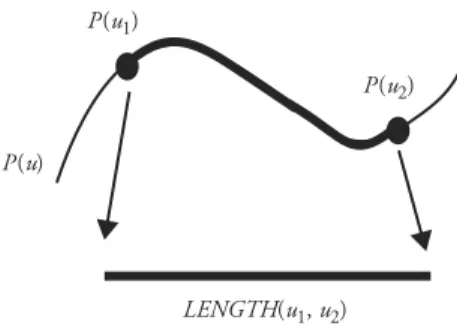
The length of the curve from a point P(u1) to any other point P(u2) can be found by evaluating the arc length integral [25] (Equation 3.3). The arc length of the curve segment from the start of the curve to the point is equal to s(t) (within some tolerance). In the following discussion, the usual assumption is that the entire arc length of the curve must be traversed during the total time given.

Figure 3.6 LENGTH(u 1 , u 2 )

Interpolation of Rotations Represented by Quaternions

Given two orientations represented by unit quaternions, intermediate orientations can be produced by interpolating linearly from the first to the second. These orientations can be seen as four-dimensional points on a straight-line path from the first quaternion to the second quaternion. The same procedure can be used to construct the Bezier curve in four-dimensional spherical space.

Figure 3.22 Equally spaced linear interpolations of straight-line path between two points on a circle generate unequal spacing of points after projecting onto a circle

Path Following

• Orientation along a Path
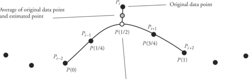
• Smoothing a Path
• Determining a Path along a Surface

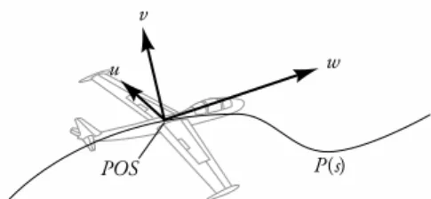
For example, the horizontal component (component in the x-z plane) of the u-axis can be used as a direction/magnitude indicator for bank. If the camera position on a curve is defined by P(s), then the center of interest will be P(s + δs). To remove deadlock, the data coordinate values ​​can be smoothed by one of several approaches.

Figure 3.29 Camera-based local coordinate system

Key-Frame Systems

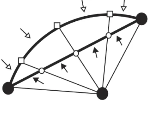
However, what happens at intermediate points along the curve has so far been left undefined (except for the obvious assumption that the entire curve P. Figure 3.50 Egg splashing against a wall whose shape must be interpolated. The first step is to create a segment of the curve to interpolate, bounded above and below by interpolation constraints. For example, tangent information along the curves can be extracted from the curve definitions.

Figure 3.49 Simple key and intermediate frames

Animation Languages

• Artist-Oriented Animation Languages
• Articulation Variables
• Graphical Languages
• Actor-Based Animation Languages

As May [28] points out, "By eliminating the language constructs that make learning animation languages ​​difficult, [artist-oriented] languages ​​give up the mechanisms that make animation languages ​​powerful." The developers found themselves adding loop constructs, conditional control statements, random variables, procedure calls, and data structure support. Reynolds [34] popularized the use of the term actor in reference to the encapsulated models he uses in his ASAS system. The current status of the actor can be extracted by a request to send information to the actor and receive a message from the actor.

Figure 3.54 Sample Houdini dataflow network and the object it generates

Deforming Objects

• Warping an Object
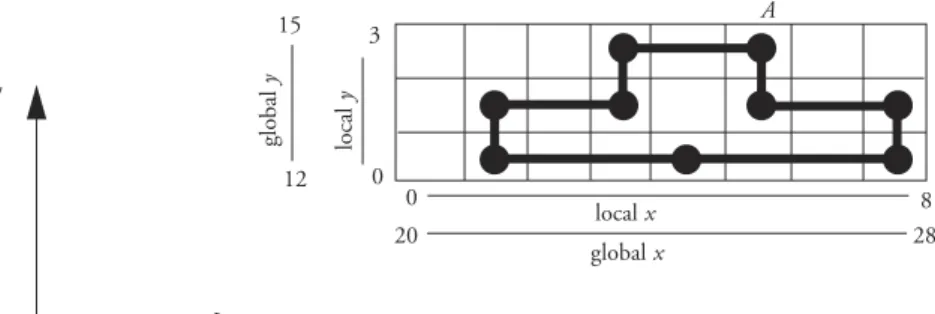
• Coordinate Grid Deformation

Moving the tool One way to animate the object is to specify the movement of the figure. 3.72 Simple example of hierarchical FFDs. Another way to animate an object using FFDs is to animate the FFD's control points. To respond to kinematic motion, the center of the FFD is fixed relative to the figure's skeleton.

Figure 3.57 Initial 2D coordinate grid

Morphing (2D)

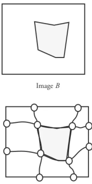
• Coordinate Grid Approach
• Feature-Based Morphing

The mapping is used on the source image to find the source image pixel that corresponds to the intermediate image pixel. This gives the displacement from the intermediate pixel to its corresponding position in the source image. For any of the intermediate frames, the feature line causes a map backward to the source image and forward to the destination image.

Figure 3.80 illustrates the formation of the auxiliary grid from the source image grid and the intermediate grid

3.9 3D Shape Interpolation

• Matching Topology
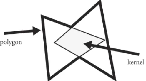
• Star-Shaped Polyhedra
• Axial Slices
• Map to Sphere
• Recursive Subdivision
• Summary
• Chapter Summary

The first meaning, from traditional mathematics, is the connectivity of the surface of an object. In the three-dimensional case, polygon definitions must then be formed on the surface of the object. Kinematic control refers to the movement of objects, regardless of the forces involved in their production.

Figure 3.88 Star-shaped polygon and corresponding kernel

Advanced Algorithms

Automatic Camera Control

If a group of objects move together, the average of their locations can be used as the camera's center point. The closest point on the constraining element to the center of interest can be calculated and used as the camera location. Fixing the camera or center of interest with a spring and damper, rather than rigidly, can help smooth out the movement.

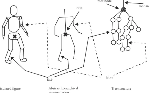
Hierarchical Kinematic Modeling

• Representing Hierarchical Models

The camera can closely follow a roaming object by establishing the camera's position relative to the moving object. A node of the tree structure contains the information needed to define the part of the object in a position ready to be articulated. This transformation also applies to the rest of the link further down the hierarchy.

Figure 4.3 Example of a tree structure representing a hierarchical structure