Credit Programmes for the Poor and Seasonality in Rural Bangladesh

(1)

The Journal of Development Studies

Publication details, including instructions for authors and subscription information:

http://www.tandfonline.com/loi/fjds20

Credit Programmes for the Poor and Seasonality in Rural Bangladesh

M.M. Pitt & S.R. Khandker Published online: 29 Mar 2010.

To cite this article: M.M. Pitt & S.R. Khandker (2002) Credit Programmes for the Poor and Seasonality in Rural Bangladesh, The Journal of Development Studies, 39:2, 1-24, DOI:

10.1080/00220380412331322731

To link to this article: http://dx.doi.org/10.1080/00220380412331322731

PLEASE SCROLL DOWN FOR ARTICLE

Taylor & Francis makes every effort to ensure the accuracy of all the information (the

“Content”) contained in the publications on our platform. However, Taylor & Francis, our agents, and our licensors make no representations or warranties whatsoever as to the accuracy, completeness, or suitability for any purpose of the Content. Any opinions and views expressed in this publication are the opinions and views of the authors, and are not the views of or endorsed by Taylor & Francis. The accuracy of the Content should not be relied upon and should be independently verified with primary sources of information. Taylor and Francis shall not be liable for any losses, actions, claims, proceedings, demands, costs, expenses, damages, and other liabilities whatsoever or howsoever caused arising directly or indirectly in connection with, in relation to or arising out of the use of the Content.

This article may be used for research, teaching, and private study purposes. Any substantial or systematic reproduction, redistribution, reselling, loan, sub-licensing, systematic supply, or distribution in any form to anyone is expressly forbidden. Terms

& Conditions of access and use can be found at http://www.tandfonline.com/page/

terms-and-conditions

(2)

Credit Programmes for the Poor and Seasonality in Rural Bangladesh

M A R K M . P I T T and S H A H I D U R R . K H A N D K E R

This article examines the effect of group-based credit used to finance self-employment by landless households in Bangladesh on the seasonal pattern of household consumption and male and female labour supply. This credit can help smooth seasonal consumption by financing new productive activities whose income flows and time demands do not seasonally covary with the income generated by existing agricultural activities. The results, based upon 1991/92 survey data, strongly suggest that an important motivation for credit programme participation is the need to smooth the seasonal pattern of consumption and male labour supply. It is only the extent of lean season consumption poverty that selects household into these programmes. In addition, the largest female and male effects of credit on household consumption are during the lean season.

I . I N T R O D U C T I O N

This article examines the effect of group-based credit for the poor in Bangladesh on the seasonal pattern of household consumption and male and female labour supply. Like much of South Asia, Bangladesh has a marked seasonal pattern of agricultural production that results in large differences in the levels of income, consumption and demand for labour across seasons.

Household members are typically engaged in agricultural pursuits and the weather induced seasonality of the crop cycle is the greatest source of seasonality in income flows.¹If seasonal income fluctuations are perfectly predictable, and if credit markets are perfect, then perfectly forecasted income changes arising from seasonal weather variations should not induce changes in consumption across seasons.

Mark M. Pitt, Brown University and Shahidur R. Khandker, World Bank, Washington, DC;

email: [email protected]. This research was funded by the World Bank project ‘Impact of Targeted Credit Programs on Consumption Smoothing and Nutrition in Bangladesh’ under research grant RPO 681-09.

The Journal of Development Studies, Vol.39, No.2, December 2002, pp.1–24 P U B L I S H E D B Y F R A N K C A S S , L O N D O N

Downloaded by [Columbia University] at 14:17 10 December 2014

(3)

However, it is not likely that credit markets are perfect in rural Bangladesh. The group-based micro-credit programmes examined below provide production credit to rural households lacking significant physical assets. These primarily agricultural households, wishing to reduce seasonal fluctuations in consumption, may try to diversify into non-agricultural activities that are less tied to seasonal weather patterns but may be credit constrained. The majority of borrowers from the micro-credit programmes studied below use their loans to finance non-farm activities. If smoothing seasonal consumption is an important motivation for poor rural households, they are likely to choose self-employment activities that generate income streams that do not highly covary seasonally with income from agricultural pursuits.

There may also be unpredictable shocks to income. Lacking the ability to formally insure against bad income realisations, households seek insurance substitutes. Transfers between households play an important role in smoothing consumption ex-post. Rosenzweig [1988] finds that net transfers flow to households that receive bad income realisations, partially taking the place of insurance markets. Diversifying income sources can not only reduce seasonal consumption variation but also reduce the effect of weather shocks on income. Farm households may cultivate different plots that are spatially separated so as to reduce the probability of being affected by common shocks, or plant different crops that are differentially susceptible to weather shocks. Households can also alter the composition of productive and non- productive asset holdings in response to the degree of weather risk.

Rosenzweig and Binswanger [1993] find that the asset portfolios of Indian farmers reflect, in part, their aversion to risk. They find there is a significant trade-off between profit variability and average profit returns to wealth and that the loss of efficiency associated with structuring one’s portfolio to mitigate risk is considerable for less wealthy farmers. Subsequent work by Rosenzweig and Wolpin [1993] examines the role of productive assets, bullocks in particular, in the risk-coping strategies of low-income farm households. They find that sales of bullocks increase when weather outcomes are poor and purchases rise when weather outcomes are favourable and that consumption smoothing is an important motivation for bullock acquisition.

In addition to its role in smoothing consumption arising from predictable seasonal variations in income, credit can also serve an insurance function much like transfers. By providing access to credit, even monitored production credit, these micro-credit programmes can help households diversify income and free up other sources of financing that can be used to directly smooth consumption. The three group-based credit programmes examined are the major micro-credit programmes in Bangladesh.

2

(4)

Participation in these programmes requires that the area of land owned should not exceed one-half acre and that ownership of other assets be of comparable magnitude. Monitored production credit is unlikely to be a perfect substitute for access to consumption credit for the purpose of smoothing consumption. Peer monitoring in these group-based programmes is sufficiently close that households may have to carry out the funded project using the borrowed funds and the participant’s time input as described in the application to borrow, even if both time and funds would be allocated differently in the absence of monitoring.

However, even perfect monitoring does not necessarily mean that production credit is not used for consumption or other purposes. If a household wishes to devote resources obtained from savings, inter- household transfers, or borrowing from moneylenders or other source to a production activity in the absence of group-based credit, it may, in the presence of group-based lending programmes, substitute group-based credit for those resources, thus freeing up those funds for other uses. In this way, simply by relaxing the household’s constraints on borrowing and transfers, monitored production credit may help households smooth consumption.

This article estimates the impact of participation, by gender, on the seasonality of household consumption and women’s and men’s labour supply for three group-based credit programmes: Grameen Bank, Bangladesh Rural Advancement Committee (BRAC), and Bangladesh Rural Development Board’s (BRDB) Rural Development RD-12 programme. In recent years, governmental and non-governmental organisations in many low income countries have introduced credit programmes such as these targeted to the poor. Many of these programmes specifically target women based on the view that they are more likely to be credit constrained than men, to have restricted access to the wage labour market, and to have an inequitable share of power in household decision-making.

The Grameen Bank of Bangladesh is perhaps the best-known example of these small-scale production credit programmes for the poor. The Grameen Bank, founded in 1976 by Muhammad Yunus, an economics professor, provides financing for non-agricultural self-employment activities. By the end of 1994, it had served more than two million borrowers, 94 per cent of whom were women [Khandker et al., 1995a].

With loan recovery rates of over 90 per cent, the Grameen Bank has been touted as among the most successful credit programmes for the poor and its model for group lending has been used for delivering credit in over 40 countries.

All three of the Bangladesh programmes examined below work exclusively with the rural poor. Although the sequence of delivery and the provision of inputs vary some from programme to programme, all three 3

(5)

programmes essentially offer production credit to the landless rural poor (defined as those who own less than half an acre of land) using peer monitoring as a substitute for collateral.²For example, the Grameen Bank provides credit to members who form self-selected groups of five.³Loans are given to individual group members, but the whole group becomes ineligible for further loans if any member defaults. The groups meet weekly to make repayments on their loans as well as mandatory contributions to savings and insurance funds. Programmes such as the Grameen Bank, BRAC and BRDB also provide non-credit services in areas such as consciousness- raising, skill development training, literacy, bank rules, investment strategies, health, schooling, civil responsibilities, and altering the attitude of and toward women.⁴

In a previous paper [Pitt and Khandker, 1998], we find that participation in these credit programmes, as measured by quantity of borrowing, is a significant determinant of women’s and men’s labour supply and household consumption. We also reject the hypothesis that programme credit is exogenous in the determination of household consumption and men’s labour supply. That is, unobserved variables that affect credit programme participation (as measured by borrowing) also affect consumption and men’s labor supply conditional on credit program participation. However, in that paper, we allowed for seasonality only by including seasonal dummy variables in the conditional demand equations. We did not allow for the effects of programme credit to vary by season. Moreover, if smoothing consumption across seasons is an important motivation for participating in these credit programmes, households with more than average seasonal fluctuations in consumption and labor supply would be more likely to participate.

This suggests that the correlation between the unobserved determinants of programme credit and consumption and labour supply may vary in intensity seasonally. In particular, our earlier work found that there was a significant and negative correlation between programme credit residuals and per capita consumption residuals implying that consumption-poor households (conditional on all the included regressors) were more likely to participate in group-based credit programmes. If seasonal consumption smoothing were a motivation for credit programme participation, we should expect that the correlation between low season consumption and credit would be bigger in absolute value (that is, more negative algebraically) than the correlation between high season consumption and credit. The results reported below find exactly this pattern. We find that the only self-selection into these credit programmes with respect to consumption expenditure arises from heterogeneity in ‘hungry season’ (Aus) consumption expenditure. It is the extent of lean season poverty that selects household 4

(6)

into these programmes.

The estimation method used in this study mirrors that set forth in Pitt and Khandker [1998].⁵The method applied corrects for the potential bias arising from unobserved individual-, household- and village-level heterogeneity.

The study uses a quasi-experimental survey design to provide statistical identification of programme effects in a maximum likelihood framework.

The survey design covers one group of households which has the choice to enter a credit programme and which may alter their behaviour in response to the programme, and a ‘control’ group which is not given the choice of entering the program but whose behavior is still measured. Furthermore, our earlier study found that credit provided to women was more likely to influence consumption and labour supply differently than credit provided to men. Thus, it is important to distinguish credit effects by the gender of the participant.

The identification of these programmes’ impact by the gender of the participant is accomplished based on the comparison between groups of each gender with and without the choice to participate. Analysing programme impacts by comparing households in villages with programs and households in village without programmes suffers from the possibility that programme placement is endogenous. These programmes, whose professed goal is to better the lives of the poor, may have chosen villages in a conscious manner based on their wealth, attitudes or other attributes. We use a village-level fixed-effects method to circumvent the problem of village unobservables biasing our estimate of the impacts of these credit programmes.

I I . E S T I M AT I O N S T R AT E G Y

Identification from a Quasi-experiment

The econometric methods used in our analysis are essentially the same as that presented in Pitt and Khandker [1998] and hence we present only an abbreviated version here. This article estimates the conditional demands for a set of household behaviours, conditioned on the household’s programme participation as measured by the quantity of credit borrowed.⁶ Leaving seasonal considerations aside for the moment, consider the reduced form equation (1) for the level of participation in one of the credit programmes (C_ij), where level of participation is taken to be the value of programme

credit that household i in village j borrows,

where X_ij is a vector of household characteristics (for example, age and 5

ε

(1)

µ π

β

c ij ^cj ^c^ij ij

ij=X +Z + +

C

(7)

education of household head), Z_ij is a set of household or village characteristics distinct from the Xs in that they affect C_ij but not other household behaviours conditional on C_ij (see below), ß_c, and B are unknown parameters, :^cjis an unmeasured determinant of C_ijthat is fixed within a village, and g^cijis a non-systematic error that reflects unmeasured determinants that vary over households such that E(g^cij, |X_ij, Z_ij, :^cj)=0.

The conditional demand for outcome y_ij (such as girls’ schooling or women’s labour supply) conditional on the level of programme

participation C_ijis

where ß_yand *are unknown parameters, :^yjis an unmeasured determinant of y_ij that is fixed within a village, and g^yij, is a non-systematic error reflecting, in part, unmeasured determinants of y_ijthat vary over households such that E(g^yij, |X_ij, :^yj) = 0. The estimation issue arises as a result of the possible correlation of :^cj with :^yj, and of g^cij with g^yij. Econometric estimation that does not take these correlations into account may yield biased estimates of the parameters of equation (2) due to the endogeneity of credit programme participation C_ij.

The standard approach to the problem of estimating equations with endogenous regressors, such as equation (2), is to use instrumental variables. In the model set out above, the exogenous regressors Z_ij in equation (1) are the identifying instruments. Unfortunately, it is difficult to find any regressors Z_ij that can justifiably be used as identifying instrumental variables. Lacking identifying instruments Z_ij, the sample survey was constructed so as to provide identification through a quasi- experimental design.

Our sample of households includes households in villages that do not have access to a group-based credit programme. If credit programme placement across the villages of Bangladesh is attentive to the village effects :j, identifying programme effects by comparing households in non- programme villages with households in programme villages will generally result in biased estimates of programme effects if selectivity of programme placement is not controlled. Using a village fixed-effects estimation technique may remove the source of correlation between programme placement and the behaviour of interest, however, without further exogenous variation in programme availability, the credit effect is not identifiable from a sample of self-selecting households as it is captured within the village fixed effects.⁷The parameter of interest, *, the effect of participation in a credit programme on the outcome y_ij, can be identified if the sample also includes households in villages with treatment choice 6

ε

(2)

β µ

δ

ij^y

y y j ij

ij=Cij +X + +

y

(8)

(programme villages) who are excluded from making a treatment choice by random assignment or some exogenous rule. That exogenous rule in our data is the restriction that households owning more than 0.5 acres of land are precluded from joining any of the three credit programmes.⁸

There are a number of participating households in our sample that had more than 0.5 acres of land at the time of programme entry, raising the possibility of mistargeting and potential bias in econometric results relying on this targeting rule. It appears that some of this excess land is either uncultivable or marginally so. Pitt [1999] demonstrates that the value per acre of land owned by programme participating households who own more than 0.5 acres of cultivable land at the time of joining is a small proportion of that value of programme participants owning less than 0.5 acres of cultivable land at the time of joining. This suggests that programme officers are using some notion of ‘effective’ units of cultivable land in determining eligibility rather than the type of mistargeting that would result in econometric bias.

Pitt [1999] discusses this issue at length and demonstrates that treating the exogenous targeting rule to be greater than 0.5 acres provides a consistent estimator for certain types of mistargeting. He finds that application of targeting rules greater than 0.5 acres (up to 2.0 acres) actually slightly strengthens the qualitative results on the effect of credit by gender on household consumption. In that paper, the relative insensitivity of the effect of credit on consumption to functional form assumptions is also demonstrated.

To illustrate the identification strategy, consider a sample drawn from two villages – village 1 does not have the programme and village 2 does;

and, two types of households, landed (X_ij=1) and landless (X_ij=0).

Innocuously, we assume that landed status is the only observed household- specific determinant of some behaviour y_ij in addition to any treatment effect from the programme. The conditional demand equation is:

The exogeneity of land ownership is the assumption that E(X_ij,g^yij) = 0, that is, that land ownership is uncorrelated with the unobserved household- specific effect. The expected value of y_ijfor each household type in each village is:

E(y_ij| j=1, X_ij=0) = :^y1 (4a) E(y_ij| j=1, X_ij=1) = $_y+ :^y1 (4b) E(y_ij| j=2, X_ij=1) = $_y+ :^y2 (4c) 7

ε

(3)

µ β

δ

ij y ^yj ^ij^y

ij=Cij +X + +

y

(9)

E(y_ij| j=2, X_ij=0) = p*+ :^y2 (4d) where p is the proportion of landless households in village 2 who choose to participate in the programme. It is clear that all the parameters, including the effect of the credit programme *, is identified from this design. In particular, the estimator of the programme effect * is a variant of the differences-in-the-differences estimator widely applied in the general programme evaluation literature. To see this, note that an estimate of *is obtained from the following difference-in-the-difference:⁹

[E(y_ij| j=2, X_ij=0) - E(y_ij| j=2, X_ij=1)] - [E(y_ij| j=1, X_ij=0)

- E(y_ij| j=1, X_ij=1)] (4e)

To illustrate the log-likelihood maximised, consider the case of a binary treatment (I_c=1 if treatment chosen, 0 otherwise) and a binary outcome (I_y=1 if outcome is true, 0 otherwise). This is the most difficult model to identify in that non-linearity arising from the choice of an error distribution is insufficient to identify the credit effect parameter *. Distinguishing between households not having choice because they reside in a non- programme village and households residing in a programme village that do not have choice because of the application of an exogenous rule (landowning status), and suppressing the household and village subscripts i and j, the likelihood can be written as:

where M₂is the bivariate standard normal distribution, Mis the univariate standard normal distribution, :^cpare the village-specific effects influencing participation in the credit programme in programme villages, :^yp are village-specific effects influencing the binary outcome I_y in programme villages, :^yn are the corresponding village-specific effects in non- programme villages, and d_c= 2*I_c- 1 and d_y= 2*I_y- 1. The errors g^cijand g^yij are normalised to have unit variance and correlation coefficient D. Village-specific effects (:^cn) influencing the demand for programme credit are not identifiable for villages that do not have programmes.

The first part of the likelihood is the joint probability of programme participation and the binary outcome I_y conditional on participation for 8

d ) ) X + ((

+ d ) ) X + ((

+

d ) , d )d + I X + ( d , ) X + ((

= ) , , , L(

y y y n village

nonprogram y y

y p village

program choice no

y c y y c

y c p c c 2 p choice

β µ β

µ

ρ β δ

µ β ρ µ

µ δ β

Φ Φ

Φ

∑

log log

no choice programme village

non-programme village (5)

(10)

those households that are both eligible to join the programme (choice) and reside in a village with the programme (programme village). This part of the likelihood corresponds to the expectation (4d). Without regressors (Z) that influence the probability of programme participation but not the outcome I_y conditional on participation, the parameter *, the effect of credit on the outcome y, is not separately identified from the parameters :^ypand $_yfrom this part of the likelihood.

The second part of the likelihood is the (univariate) probability of binary outcome I_yfor landed households in programme villages and corresponds to expectation (4c). These households are precluded from joining the programme by their landed status. The last part of the likelihood is the probability of the outcome I_y for all households, landed and landless, in villages without a programme and corresponds to expectations (4a and 4b).

If one of the regressors in X is a binary indicator of landed status, this part of the likelihood is required for identification. If landed status is a continuous measure of landholding, then the model is identified without the last part of the likelihood. In this case, the parameter $_yin (3) is identified from variation in landholding within the programme villages (j=2) and a sample of non-programme villages is not required.

Even if land ownership is exogenous for the purposes of this analysis, it is necessary that the ‘landless’ and the ‘landed’ can be pooled in the estimation. In order to enhance the validity of this assumption, we restrict the set of nontarget households used in the estimation to those with less than 5 acres of owned land. In addition, we include the quantity of land owned as one of the regressors in the vector X_ijand include a dummy variable indicating the target/non-target status of the household.

The exclusion restrictions that identify the effects of credit on the outcomes y_ij are the interactions of a dummy variable indicating if the household has the choice to join the credit programme (which requires meeting the land ownership rule and residing in a village with a credit programme) and all the exogenous variables of the model, X_ij and :_j. Consequently, the model is not non-parametrically identified; that is, if the linear indices X_c(and (X_y$+*I_c) in (5) were replaced by non-parametric functions of the Xs, and I_cthe model is not identified.

Identification of the Impact of Gender-Specific Credit using Single-Sex Groups

An important question of this research is whether various behaviours are affected differently by credit if the program participant is a woman or a man. For that reason, the reduced form credit equation is disaggregated by gender

9

(11)

where the additional subscripts f and m refer to females and males respectively. The conditional household outcome equations allow for seasonal intercept dummy variables as well as separate female and male credit effects by season:

where D_jfs and D_jmsare village specific indicator variables such that D_jfs takes the value of one in village j in season s if there is a female group in village j, and zero otherwise.

Additional identification restrictions are required when there are both male and female credit programmes with possibly different effects on behaviour. Identification of gender-specific credit is also achieved by making use of another quasi-experimental attribute of these programmes and the survey. All programme groups are single-sex and not all villages have both a male and a female group. The sample includes some households from villages with only female credit groups, so that males in landless households are denied the choice of joining a credit programme, and some households from villages with only male credit groups, so that landless females are denied programme choice.¹⁰In particular, of the 87 villages in the sample, 15 had no credit programme, 40 had credit groups for both females and males, 22 had female-only groups and ten had male- only groups. The necessary assumption is that the availability of a credit group by gender in a village is uncorrelated with the household errors g^yij, conditional on X_ijand the village fixed effects :j. As each village had only one type of credit programme available, and it is assumed that the type of credit programme (BRDB, BRAC or Grameen) is uncorrelated with the household errors Σ^y_ij, conditional on X_ij and the village fixed effects :_j, there is no need to model which of the programs members of a household join.¹¹

While the likelihood given by (5) illustrates the general principle and method used, the actual likelihoods maximised have been altered to allow for other aspects of our data. Male and female credit and the labour supply of women are limited dependent variables with a mass point at zero.

Consequently, the likelihoods contain trivariate normal distribution functions because two credit equations (6) and (7) are being estimated simultaneously with a limited dependent variable outcome equation. In addition, the sample design is choice-based (see section III below). In particular, programme participants are purposely over-sampled.

10

ε

(6)

µ

β

cf ^cjf ^c^ijf ij

ijf = X + +

C

ε

(7)

µ

β

ijm^c

c jm ij cm

ijm

= X + +

C

ε (8) δ δ

µ α

β ^ijm ^jms ^ms ^ijs^y

s fs ijf jfs s jfs s s y j ijs y

ijs=X + + D + C D + C D +

y

∑ ∑ ∑

(12)

The Weighted Exogenous Sampling Maximum Likelihood (WESML) methods of Manski and Lerman [1977] were grafted on to the limited information maximum likelihood (LIML) methods described above in the estimation of both parameters and the parameter covariance matrix.¹² WESML estimates are obtained by maximising a weighted log likelihood function with weights for each choice equal to the ratio of the population proportion to the sample proportion for that choice. To remind the reader of these crucial aspects of the maximum likelihood approach taken in this analysis, the method is referred to as WESML-LIML-FE, which stands for Weighted Exogenous Sampling Maximum Likelihood – Limited Information Maximum Likelihood – (Village) Fixed Effects. Pitt and Khandker [1998] provide an explicit characterisation of the likelihood actually maximised as well as the asymptotic covariance matrix.

The specifications of the conditional demand for consumption and conditional labour supply equation presented here differ from those in Pitt and Khandker [1998] in that credit effects are allowed to vary by season, and the correlation between the residuals of these equations and the male and female credit equations are also allowed to vary seasonally. In addition, we do not discriminate among the three credit programmes in the estimates below. Our earlier work found no significant difference in the effects of borrowing from BRDB, BRAC and the Grameen Bank on labour supply and household consumption.

I I I . D ATA , S U RV E Y D E S I G N A N D T H E N AT U R E O F S E A S O N A L I T Y I N B A N G L A D E S H

A multi-purpose quasi-experimental household survey was conducted in 87 villages of 29 thanas in rural Bangladesh during 1991–92. The sample consists of 29 thanas (sub-districts) randomly drawn from 391 thanas in Bangladesh, of which 24 had one (or more) of the three credit programmes under study in operation, while five thanas had none of them.

Three villages in each programme thana were then randomly selected from a list of villages, supplied by the programme’s local office, in which the program had been in operation at least three years. Three villages in each non-program thana were randomly drawn from the village census of the Government of Bangladesh. A household census was conducted in each village to classify households as target (that is, those who qualify to join a program) or non-target households, as well as to identify programme participating and non-participating households among the target households.

A stratified random sampling technique was used to over-sample households participating in one of the credit programmes and target non-participating households. Of the 1,798 households sampled, 1,538 were target households 11

(13)

and 260 non-target households. Among the target households, 905 households (59 per cent) were credit programme participants.

There are six partly overlapping seasons delineated in the Bangla calendar and three major rice-based seasons are prominent. The survey of households and communities was designed to reflect this pattern of seasonality. The survey was carried out in three rounds corresponding to the Aus, Aman and Boro cropping seasons. The first round of the survey was conducted during the months of December–January, during the post-harvest of Aman rice. The second round of survey was carried out during the months of April–May to cover the post-harvest season of Boro rice. The third round of the survey was carried out during the months of July–August to cover the post-harvest of Aus rice. In our sample survey data, season one refers to the Aman season, season two refers to Boro season, and the season three refers to the Aus season.

The strong seasonality of crop production in Bangladesh is well known to affect the timing of income flows. The Aman rice is the largest crop in Bangladesh agriculture and, hence, its production and harvest has the largest impact on agricultural employment, income and prices. Both Boro and Aus also provide enhanced opportunities for employment but not in the same scale as Aman. As the use of high-yielding varieties and irrigation technologies has spread, Boro crop production has increased in recent years.

None the less, the period of least food consumption for the rural poor has traditionally taken place in the months just before the Aman harvest. The food availability on a per capita basis is the highest during the months just after the Aman harvest (November–December), and also during May–June, just after the harvest of Boro rice [Chowdhury, 1989].

Agricultural employment also responds to seasonal variations in the demand for labour in various crop-related activities. The Aman harvest during the months of November–December is characterised by the greatest demand for agricultural labour. The labour demand is also relatively high in the months of January and March, when the transplantation of Boro HYV takes place. Labor demand is lowest during the months of September–

October just before the harvest of Aman rice. This seasonality in labour demand is mirrored by the seasonal pattern of agricultural employment and wages, and consequently, in the seasonal consumption landless households who depend heavily on wage employment. [Muqtada, 1975; Hossain, 1990].

Table 1 presents the weighted mean and standard deviations of all the dependent variables used in the regression, by season. Because the samples drawn are not representative of the village population, the means of the variables are adjusted by appropriate weights based on the actual and sample distribution of the households covered in the study villages. The exogenous variables include a set of variables indicating the existence of 12

(14)

TABLE 1 WEIGHTED MEANS AND STANDARD DEVIATIONS OF DEPENDENT VARIABLES Dependent VariablesHouseholdsObs.HouseholdsObs.AllObs.HouseholdsObs.AllObs. withwithouthouseholdsin non-households participantsparticipantsin programmeprogramme areasareas Women’s labor supply40.328342037.680210838.905552843.934107439.5406602 (hours per month, (70.478)(71.325)(70.934)(74.681)(71.432) ages 16-59 years) Season 1 (Aman)44.515115740.55972041.8555187729.12136539.8252242 (73.961)(72.661)(73.088)(67.761)(72.401) Season 2 (Boro)37.904113928.99869831.950183729.72835731.5872194 (68.590)(59.067)(62.504)(52.228)(60.939) Season 3 (Aus)38.492112427.69369031.290181435.00135231.9012166 (68.549)(59.213)(62.664)(59.895)(62.519) Men’s labor supply202.7583534185.8582254191.3105788180.941126189.4776914 (hours per month,(100.527)(104.723)(103.678)(98.805)(102.902) ages 16-59 years) Season 1 (Aman)209.3891201196.037769200.3301970184.352383197.5262353 (107.000)(112.121)(110.640)(101.847)(109.296) Season 2 (Boro)201.8491173181.772746188.2671919190.737372188.7042291 (96.821)(100.899)(100.007)(96.384)(99.530) Season 3 (Aus)196.8481160179.435739185.0551899167.651371181.9612270 (96.942)(99.808)(99.193)(95.853)(98.810) Weekly per capita77.014269685.886165082.959434689.66187284.0725218 HH total expenditure (Taka)(41.496)(64.820)(58.309)(66.823)(59.851) Season 1 (Aman)87.67390595.16255792.706146284.03829591.2681757 (50.837)(63.754)(59.901)(50.555)(58.530) Season 2 (Boro)79.40789788.85754885.7321445111.15229089.9651735 (39.808)(59.411)(53.883)(94.469)(63.177) Season 3 (Aus)63.87289473.41354570.253143973.70728770.8261726 (26.470)(34.459)(58.695)(34.459)(55.419) Note:Standard deviations are in the parentheses.

(15)

nonresident relations of various type who are landowners. These types of households are potential sources of transfers which may importantly substitute for credit.

The strong seasonality of labour supply and weekly per capita household consumption is evident in Table 1.¹³Women’s Aman season labour supply is about 25 per cent higher than Boro and Aus season labour supply. Men’s labour supply is highest in the Aman season, five per cent lower in the Boro season, and eight per cent lower than in the Aus season. The imperfect ability of household to smooth consumption is also clearly seen in Table 1.

Average consumption in our 1991/92 sample is highest in the Aman season, is only 2.5 per cent lower in the Boro season but is a striking 22.5 per cent lower in the Aus season.

I V. E C O N O M E T R I C R E S U LT S

14

TA B L E 2

A LT E R N AT I V E E S T I M AT E S O F T H E I M PA C T O F C R E D I T O N P E R C A P I TA E X P E N D I T U R E A N D W O M E N ’ S A N D M E N ’ S L A B O R S U P P LY

Explanatory Log of Weekly Women’s Labor Supply: Men’s Labor Supply:

Variables Total Expenditure Hours in past month Hours in past month per Capita

WESML- WESML- WESML- WESML-

LIML-FE FE LIML-FE LIML-FE

Amount borrowed by .0394 0.0721 -.0117 -.1813

female from BRAC (4.237) (1.884) (-.128) (-5.884)

Amount borrowed by .0192 -.0126 -.0448 -.1369

male from BRAC (1.593) (-.231) (-.520) (-2.155)

Amount borrowed by .0402 .0766 -.0139 -.2308

female from BRDB (3.813) (1.803) (-.139) (-7.066)

Amount borrowed by .0233 .0268 -.0144 -.1440

male from BRDB (1.936) (.682) (-.181) (-2.129)

Amount borrowed by .0432 .1037 .0152 -.2189

female from GB (4.249) (3.016) (.162) (-6.734)

Amount borrowed by .0179 -.0229 -.0570 -.1592

male from GB (1.431) (-.506) (-.677) (-2.524)

Season 2 (Boro) -.0178 -.311 -.315 -.0384

(-1.276) (-2.150) (-2.169) (-.823)

Season 3 (Aus) -.232 -.239 -.242 -.0908

(-17.083) (-1.511) (-1.534) (-2.174)

D (women) -.4809 .1255 .6564

(-4.657) (1.062) (7.461)

D(men) -.2060 .0560 .4929

(-1.432) (.592) (2.512)

Log likelihood -6633.559 -15071.59 -15069.781 -18395.082

No. of observations 5218 6602 6602 6914

Note: Figures in parentheses are asymptotic t-ratios.

Source: Pitt and Khandker [1998].

(16)

Table 2 excerpts the estimates of the determinants on the natural logarithm of total weekly expenditure per capita, and women’s and men’s labour supply, conditional on programme credit, that were estimated and presented in Pitt and Khandker [1998]. Over 200 parameters are jointly estimated in each case and we only present the estimated credit effects, correlation coefficients and seasonal dummies. The null hypothesis of credit exogeneity is rejected for both expenditure and men’s labour supply, so the WESML- LIML-FE estimates, which treat both village programme placement and household and individual participation as endogenous, are the preferred specifications. Exogeneity of household and individual credit programme participation cannot be rejected in the case of women’s labour supply, and so the WESML-FE estimates, which treat only programme placement as endogenous, are the preferred estimates.

The estimates of the impact of credit programme participation on the natural logarithm of total weekly expenditure per capita using all three rounds of survey data, presented in Table 2, reveal that female credit parameters are positive and statistically significant determinants of total expenditure, with no t-statistic less than 3.8, and are jointly significant (χ²(3)=19.03, p=0.00). In contrast, none of the male credit parameters has a t-statistic over 2.0 and the hypothesis that all the male credit parameters are zero cannot be rejected at the 0.05 level of significance (χ²(3)=4.11, p=0.25). The estimated female credit effects are approximately double the male credit parameters for the same credit programme.¹⁴

There are not substantially different effects among the three credit programmes. At the mean, an additional one taka of credit provided participating women adds 0.18 taka to total annual household expenditure, as compared with 0.11 taka if the same amount of additional credit is supplied to participating men. The WESML-LIML-FE Ds are both negative, more so for women, suggesting that, conditional on their village of residence and observed characteristics, low expenditure households are more likely to participate in a credit programme. That is, poorer households are being successfully targeted. The seasonal dummy variables demonstrate highest consumption in the Aman round (season 1) of the survey and significantly lower consumption in the Aus season (season 3), as expected.

The WESML-FE women’s labour supply estimates demonstrate a statistically significant positive effect of women’s participation in the Grameen Bank on women’s labour supply, and the marginal significance of the women’s BRAC and BRDB parameters. As both labour supply and credit are in natural logarithms, the credit parameters are the elasticities of (latent) hours of market labour supply with respect to credit. The pattern of dummy variables in the women’s labour supply equation suggests that Aman labour supply is highest and Boro season labour supply is the smallest, conditional on the regressors.

15

(17)

The male labour supply estimates suggest that both male credit (χ²(3)=98.66, p=0.00) and female credit (χ²(3)=53.11, p=0.00) reduce the labour time of adult male household members. A ten per cent increase in male group-based credit is associated with about a 1.4 per cent decline in labour supply, and a ten per cent increase in female group-based credit is associated with about a 2.1 per cent decline in labour supply. As it seems unlikely that they are substituting home time for market time, the only conclusion to be drawn is that these negative cross-effects reflect income effects.

If the market value of men’s time is unchanged by women’s borrowing, their labour supply should fall if male leisure is a normal good. This is consistent with a variety of scenarios. One of these is that men already have ready access to non-program credit markets, so that program credit mostly provides men with rents proportional to the difference between the programme and next-best-alternative rates of interest.¹⁵These labour supply results suggest that one other reason the effect of programme credit on total household expenditure on goods is higher for women than men is the increased consumption of leisure associated with male borrowing. As with women, the pattern of seasonal intercept suggest the Aman season as the season of greatest labour supply, but unlike women, labour supply is least in the Aus season.

Table 3 presents alternative estimates of the seasonal effects of credit on per capita expenditure. The first column presents estimates like those in Table 2 except that credit effects are allowed to vary by season but not by credit programme. The effect of both female and male credit on consumption expenditure is greatest in the Aman season, the season of greatest expenditure, suggesting that programme credit may not reduce the seasonal fluctuation in consumption. However, these estimates restrict the correlation (ñ) between credit and consumption residuals to be constant across the seasons, which we have argued is unlikely to be true if one motivation for joining these credit programmes is the need to smooth consumption across the seasons, and there is seasonal heterogeneity in the population.

The estimates of column 2 in Table 3, in which ñ is allowed to vary by season, tell a completely different story. The largest effect of female credit on consumption is during the Aus season, the season of lowest average consumption, although Aman effects are not much lower. For male credit, restricting ñ to not vary across seasons results in an underestimate of both Aman and Aus season credit effects. Underlying this is the large ñ associated with the Aus season for both women and men, suggesting that households with low consumption (conditional on the observed regressors) during the Aus season are more likely to participate and borrow from these credit programme than households with low consumption expenditure in the other seasons.

16

(18)

The last three columns of Table 3 present estimates of the effects of programme credit on consumption expenditure in which all the parameters, not just credit effects and Ds, are allowed to vary by season. These estimates are obtained by estimating our model one season at a time. These estimates provides even more striking evidence on the importance of seasonality in evaluating the effect of credit programmes on the poor. The only statistically significant correlation coefficients (D) are for the low consumption Aus season. Apparently, self-selection into these credit programmes with respect 17

TA B L E 3

A LT E R N AT I V E E S T I M AT E S O F T H E I M PA C T O F C R E D I T O N T H E S E A S O N A L PAT T E R N O F L O G W E E K LY P E R C A P I TA E X P E N D I T U R E

WESML-LIML-FE estimates

Explanatory Variables Pooled Pooled Season 1 Season 2 Season 3

Amount borrowed by .0453 .0432 .0313

female x season 1 (Aman) (4.634) (5.156) (1.206)

female x season 2 (Boro) (3.899) (3.370) (1.580)

female x season 3 (Aus) (4.002) (5.827) (4.879)

male x season 1 (Aman) (2.225) (2.690) (.238)

male x season 2 (Boro) (1.433) (.935) (1.042)

male x season 3 (Aus) (1.408) (1.828) (1.861)

Season 2 (Boro) .00155 .00886

(.087) (.387)

Season 3 (Aus) -.214 -.234

(-12.217) (-11.179)

D(women) -.478

(-4.485)

D(men) -.206

(-1.393)

D(women, season 1) -.437 -.339

(-4.746) (-1.046)

D(women, season 2 ) -.429 -.410

(-3.314) (-1.577)

D(women, season 3) -.606 -.568

(-7.495) (5.906)

D(men, season 1) -.237 .0423

(-1.797) (.137)

D(men, season 2) -.106 -.144

(-.621) (-.797)

D(men, season 3) -.304 -.272

(-1.985) (2.015)

Log likelihood -6631.00 -6623.56 -2160.34 -2191.23 -1992.06

No. of observations 5218 5218 1757 1735 1726

(19)

to consumption expenditure arises only from heterogeneity in Aus consumption expenditure. It is the extent of lean season poverty that selects household into these programs. Not surprisingly, the largest female and male effects are during the lean Aus season. Given the much larger number of parameters that are estimated in this model, the precision of our estimates falls as compared to the first two columns of the table. Only women’s credit during the Aus season has a t-ratio greater than 2.0.

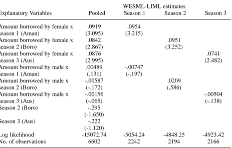
Table 4 presents our new estimates of the seasonal effect of credit on women’s labour supply. Programme credit was found to be exogenous in the determination of women’s labour supply in our earlier work, and that finding persists in the seasonal specifications. It is harder to unambiguously relate the pattern of parameter estimates presented in Table 4 to a need to smooth the seasonal pattern of market labour supply. Women’s market labour supply is only one-sixth that of men, and so we are not looking at the

most important use of their time when we examine market time. Nor do we have a clear understanding of whether the productivity of women’s nonmarket time varies by season and the extent to which there are inter- seasonal substitution possibilities in the production of nonmarket goods. It seems unlikely that there is much inter-seasonal substitution for important goods such as child care and food preparation.

18

TA B L E 4

A LT E R N AT I V E E S T I M AT E S O F T H E I M PA C T O F C R E D I T O N T H E S E A S O N A L PAT T E R N O F W O M E N ’ S L A B O R S U P P LY ( H O U R S I N L A S T M O N T H )

WESML-LIML estimates

Explanatory Variables Pooled Season 1 Season 2 Season 3

Amount borrowed by female x .0919 .0954

season 1 (Aman) (3.095) (3.215)

season 2 (Boro) (2.867) (3.252)

season 3 (Aus) (2.995) (2.482)

Amount borrowed by male x .00489 -.00747

season 1 (Aman) (.131) (-.197)

Amount borrowed by male x -.00587 .0209

season 2 (Boro) (-.172) (.586)

Amount borrowed by male x -.00156 -.00504

season 3 (Aus) (-.065) (-.138)

Season 2 (Boro) -.295

(-1.650)

Season 3 (Aus) -.222

(-1.120)

Log likelihood -15072.74 -5054.24 -4848.25 -4923.42

No. of observations 6602 2242 2194 2166

(20)

It is interesting to note that in the non-programme villages of our sample, Aus season labour supply is about 20 per cent greater than in the Aman and Boro seasons, but in the programme villages, Aman season women’s labour supply is substantially higher than in both the Boro and Aus seasons. This different pattern may to some extent reflect the effects of the credit programmes on the seasonal distribution of market time allocation in the village as a whole, as well as non-random programme placement across villages and sample variation. The estimates in column 1 of Table 4 do not 19

TA B L E 5

A LT E R N AT I V E E S T I M AT E S O F T H E I M PA C T O F C R E D I T O N T H E S E A S O N A L PAT T E R N O F M E N ’ S L A B O R S U P P LY ( H O U R S I N L A S T M O N T H )

WESML-LIML-FE estimates

Explanatory Variables Pooled Pooled Season 1 Season 2 Season 3

Amount borrowed by -.212 -.206 -.196

female x season 1 (Aman) (-6.832) (-6.687) (-4.047)

female x season 2 (Boro) (-6.051) (-7.391) (-10.552)

female x season 3 (Aus) (-6.252) (-5.077) (-.280)

Amount borrowed by .00207 -.0271 -.171

male x season 1 (Aman) (.184) (-.646) (-3.953)

Amount borrowed by .00148 -.0131 .0232

male x season 2 (Boro) (.155) (-.367) (.885)

Amount borrowed by -.103 -.0871 .0378

male x season 3 (Aus) (-2.032) (-1.101) (1.096)

Season 2 (Boro) -.0770 -.0627

(-1.230) (-.758)

Season 3 (Aus) -.109 -.127

(-1.951) (-1.672)

D(women) .652

(7.196)

D(men) .487

(2.237)

D(women, season 1) .629 .597

(6.233) (4.458)

(8.356) (16.595)

(5.162) (.430)

D(men, season 1) .521 .575

(2.085) (4.224)

D(men, season 2) .410 -.050

(1.093) (-.723)

D(men, season 3) .462 -.116

(1.046) (-1.026)

Log likelihood -18406.20 -18399.95 -6145.33 -6051.23 -6047.89

No. of observations 6914 6914 2353 2291 2270

(21)

suggest important differences in the effect of credit on women’s labour supply by season, consistent with the view that there is likely to be less seasonality in the time allocation of women given the small share of market time in total time. Breaking the sample by round does not qualitatively alter this finding, although the point estimate of the Aus season credit effect is about 22 per cent lower that in the Aman or Boro seasons.

In the sampled households, men devote considerable time to the market;

more than 43 hours per week in the full sample and 46 hours per week among participating households, with Aman being the peak season. The first column of Table 5, which allows credit effects to vary by season but does not allow for differential self-selection by season, does not find any seasonal variation in the effect of women’s credit, but does suggest that men’s credit reduces slack season (Boro) men’s labour supply (t=-2.03) and has no effect on labour supply in other seasons. Allowing for differential self-selection (endogeneity) by season in column 2 suggests that there is no difference in the effects of both men’s and women’s credit by season on men’s labour supply. Breaking the sample by season (columns 3 to 5), the most flexible specification of seasonal effects, suggests that there are indeed strong seasonal differences in the effect of both women’s and men credit, and in the pattern of self-selection.

Women’s credit has no statistically significant effect on men’s Boro season labour supply, but large (in absolute value), negative and statistically significant effects on men’s Aman and Boro season market labour supply.

Women’s Aman and Boro credit effects are approximately ten times the Aus credit effect. Women’s credit reduces men’s labour supply except in the slack season. In addition, the correlation coefficients (ñ) between the women’s credit error and the men’s labour supply error are only large and statistically significant during the Aman and Boro seasons, so, as with household consumption, the endogeneity of women’s programme credit is only seasonal – that is, self-selection of women into the credit programme is only seasonal with respect to men’s labour supply.

The negative effects of men’s credit on their labour supply reported in our earlier work and in Table 2 obscures important seasonal differences. In the Boro and Aus season, men’s credit has small positive but statistically insignificant effects on their labour supply. In addition, the pattern of correlation coefficients (D) reflects this seasonal pattern. There is a large positive correlation coefficient between men’s credit residuals and labour supply residuals for the Aman season, but small negative D’s for the other seasons. Men with higher than average demands on their time during the Aman season (conditional on the regressors), the time of peak labour demand, are more like to self-select themselves into these credit programmes and borrow from them, with the consequence of reduced market labour supply during that peak season.

20