Major improvements have been made to several components of the system, including the construction of a new actuator probe to decouple the in-plane and out-of-plane motions, the design and implementation of a new first stage amplifier to reduce the noise output by a factor. 10 and modeling the controller in the STM feedback loop. In the simple case of one-dimensional correlation, the main parameters involved are the subset size, variables in the displacement representation, frequency content of the signal, and noise.
List of Tables
1 Introduction
In Chapter 4, a detailed analysis is made on the nature of noise associated with AFM scans. The influence of white noise, intrinsic to AFM instruments, on correlation is revealed and a possible improvement is proposed to compensate for the hysteresis of the AFM piezo actuator.
2 The Scanning Tunneling Microscope
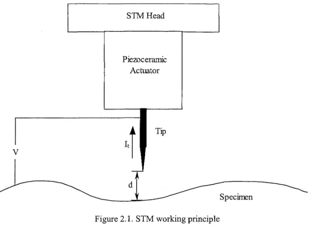
The Working Principle
- Tunneling Phenomenon
- Feedback Loop
- The Piezoceramic Actuator
The theory of the line tunneling microscope is based on the tunneling effect in quantum physics. The amount of correction required by the actuator indicates the relative height of the spot on the sample surface below the tip.
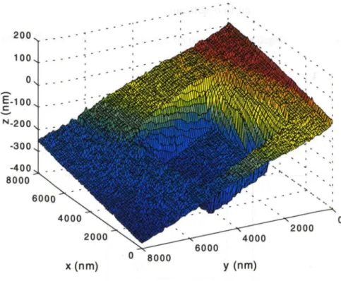
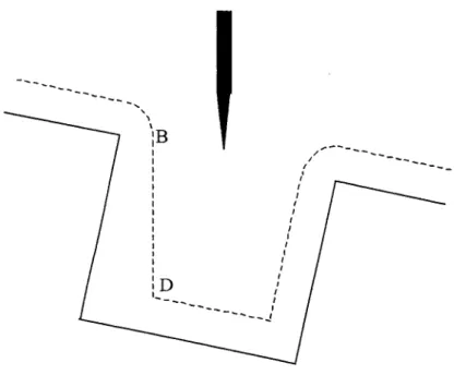
Calibration
Specifically, until point A directly above the corner of the step, the tip follows the surface profile. Depending on the length of the step, the trace may not reproduce the true depth of the step.
Hardware Improvement
- A New Actuator Probe
- The Current-to-Voltage Converter
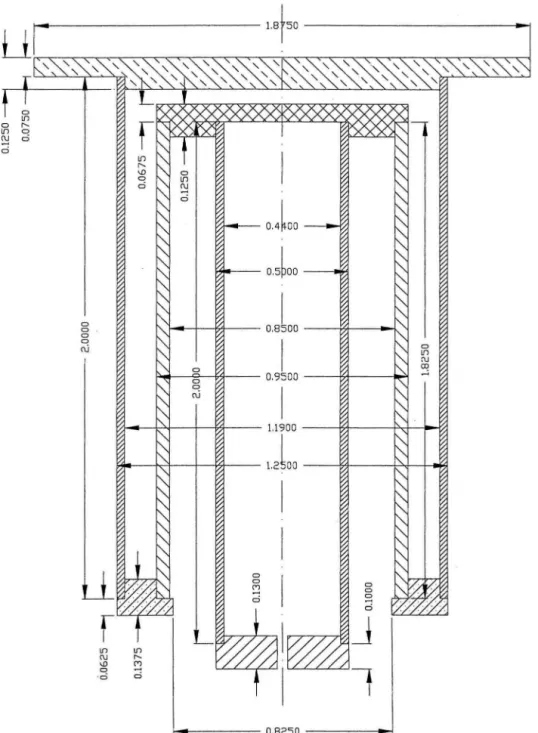
Although some problems related to piezoceramic actuator hysteresis and drift-induced noise remain, STM can perform surface measurements with submicron resolution. In Figure 2.16, the two tubes with the _ flap are piezoceramic actuators, while all other parts are made of ceramic, which has a coefficient of thermal expansion very close to that of the piezo material. There is no documentation on the response time of the piezoceramic actuator, nor could the manufacturer provide definitive information.
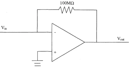
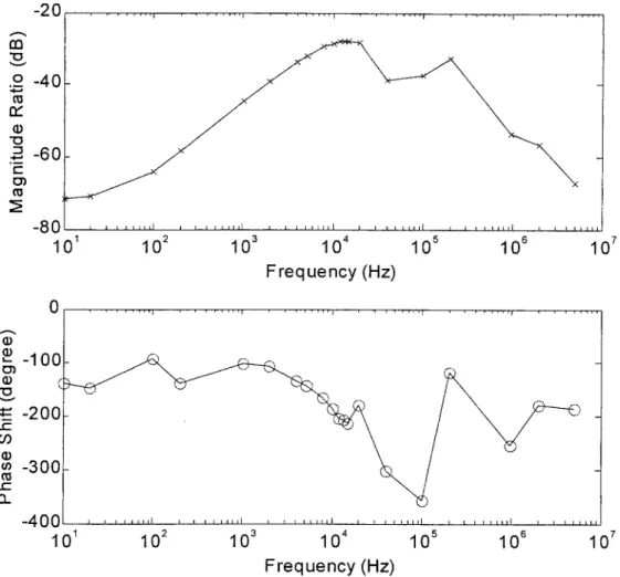
O, as shown in Figure 2.4, and measure the magnitude and phase shift of the sinusoidal output. Due to the difficulty in directly measuring the small deformations of the piezo ceramic tube, this test is performed during tunneling, and instead the output voltage is measured across a current-to-voltage converter, or Vt, as shown in Figure 2.2. Since the current-to-voltage converter actually responds about 10 times faster, this result essentially represents the response time of the piezoceramic actuator.
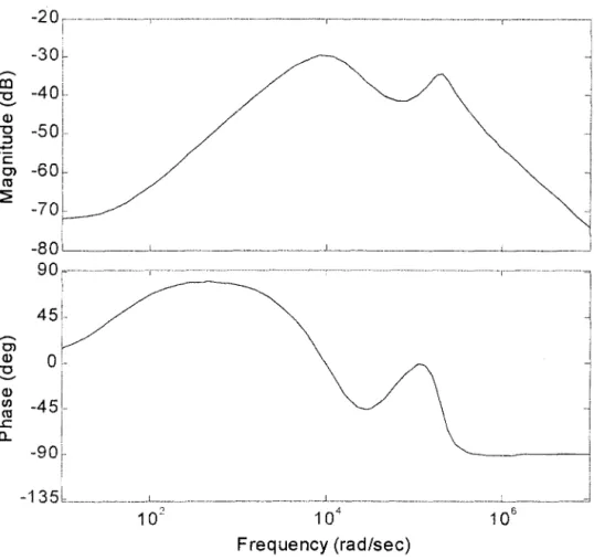
All these plots indicate that if the linear controller model represents the dynamic behavior of the actuator, the current feedback frequency set at 100kHz is clearly too fast for the piezo-ceramic actuator to respond.
Conclusion
Therefore, the modeling of the STM controller in this section is used for estimation purposes only. The first-stage amplifier that converts the tunnel current to voltage has been redesigned to incorporate three amplifiers. The new amplifiers filter out high-frequency noise and have reduced the overall noise level in the output by a factor of 10.
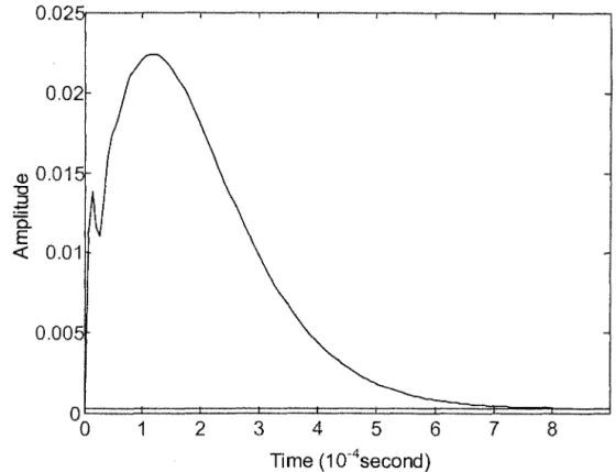
To keep the translation stage intact, the new amplifiers are installed in the existing setup in the form of a stack. To access the performance of the feedback controller, the dynamic behavior of the piezoceramic actuator was modeled using a mathematical linear controller model. Testing of the linear model controller shows that the piezoceramic actuator has a response time on the order of 0.5ms, which is slow compared to the feedback frequency of the current setting.
However, this model may not fully represent the piezoceramic actuator and can therefore only be used as a reference.
3 Digital Image Correlation
One-Dimensional Digital Image Correlation
- Theoretical Background
- Continuous Signals
- Conclusion
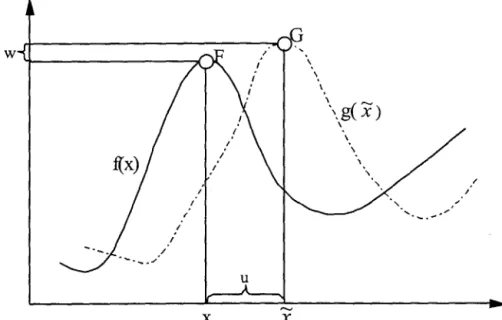
The one-dimensional correlation is first derived theoretically, based on the assumption that the deformation is small enough to preserve the characteristic features of the profile. For example, the size of the subset chosen for correlation has been recognized by researchers[13]-[l6] as a key parameter, but its effect has not been closely studied. Finally, a summary of important parameters is given and quantitative measures are proposed for a better digital image correlation.
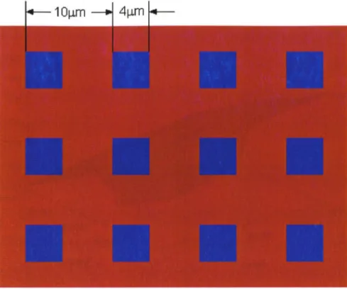
On the other hand, the subset must include some signal features so that it can be easily related to the deformed subset, which argues for a larger subset. Depending on which frequency component is dominant, the size of the subset should be equal to at least half of the longest wavelength. For this part of the study, a scanning image of a silicon surface shown in figure 3.12 was used.
This problem can be traced back to the spiky nature of the second-order gradient of the height profile used in the Hessian matrix, as shown in Figure 3.16. In numerical calculations, a small error in the Hessian matrix can cause a large difference in the solution of the linear equations. Replacing the exact Hessian matrix (3.1.14) with the approximation (3.1.15) in the correlation does not improve convergence in general.
Two-Dimensional Digital Image Correlation
- Theoretical Background
- Continuous Surfaces With Well Defined Frequency Content
- Real Scan Images
- Conclusion
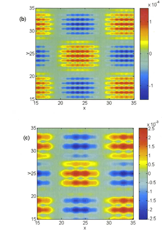
A large number of digits are deliberately included in the defined offsets to obtain the correlation error correctly. Correlation errors with only w in the displacement representation increase with greater out-of-plane propensity. From these results, we deduce that it is important to include a sufficient number of out-of-plane strain terms in the correlation expression to represent the defined displacement field so that the algorithm converges to the absolute minimum.
As shown in the previous section, this may be due to an insufficient number of sample points. The influence of more random uncertainty on the correlation process will be discussed in the next chapter. The reason is that for small subsets the quadratic term in the displacements is not dominant, so that the correlation results follow the same trend as for linear deformations.
This study on two-dimensional digital image correlation systematically identifies and evaluates the important parameters of the process. Because of interpolation, the spatial sampling rate becomes an important factor in the correlation process. The more dominant the non-linear contribution is in the deformation, the larger the correlation error.
Temporal Noise
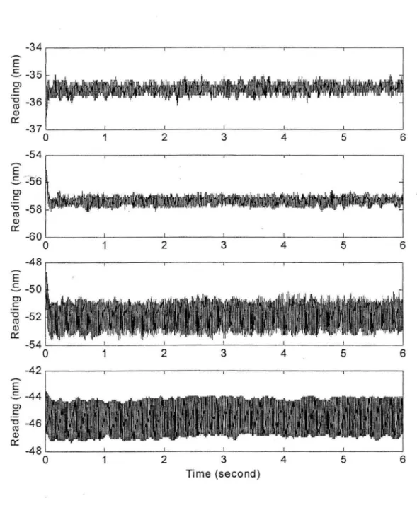
Therefore, it is important to understand the nature and characteristics of noise before its impact on digital image correlation can be fully assessed. When the AFM is in scanning mode, this temporal noise translates into inconsistency or uncertainty between repeated scans. To analyze the frequency content of the temporal noise, the Fourier transform is applied to the first record in Figure 4.1.
The initial regularity in the record is not taken into account for the frequency analysis, because it can have an influence on the analysis. The part of the signal used is shown in Figure 4.2 and its frequency spectrum is shown in Figure 4.3. The filtered signal and its frequency spectrum are displayed in the same figures for comparison.
The remaining noise is mostly white noise, with a uniform frequency distribution as shown in Figure 4.3 (b). a) Original signal, (b) Filtered signal at a cutoff frequency ~80Hz.
Spatial Uncertainty
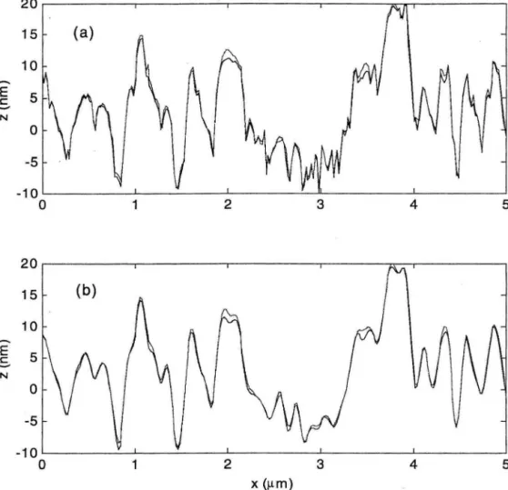
Although amplitude is small, the uncertainty between these two line profiles is not negligible when performing the digital image correlation. 34;artificial" displacements for up to half a pixel (corresponding to approximately Srun) were generated from this inconsistency of repetitive scans. This "artificial" displacement will cloud the calculation of real displacements when performing image correlation for a deformed sample.
The error is consistent with the "artificial" displacement created by the repeated line scans shown in Figure 4.6. For this particular case, the error in the displacement u from the image correlation is comparable to the magnitude of the described displacement. For example, when a uniform stress Ex=O.l is applied, the error will appear much smaller compared to the described displacement, simply because the described displacement is 10 times larger.
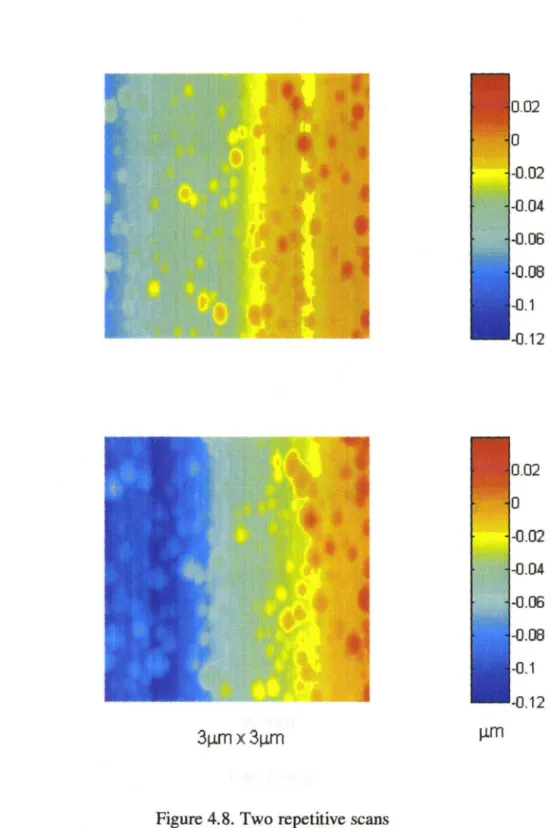
Because the uncertainty between repeated scans arises from the random temporal noise (shown in Figure 4.1) that is essential to atomic force microscopy instrumentation, it is not possible to predict the uncertainty pattern through calibrations.
Problems with Two-Dimensional Images
It can only be concluded that the displacement calculated from the AFM scans may have an error of half a pixel, but we cannot eliminate this error. However, by carefully choosing the area to be correlated (which has large displacements within the sample), the relative error can be minimized and the stresses derived more accurately. Hysteresis also develops in both plane directions, which explains the translation between the two images.
By carefully choosing the various parameters involved in the scan, the influence of hysteresis can be minimized. Therefore, it is suggested here that the AFM manufacturer follows a procedure to reduce the hysteresis effect: after each line scan, the position of the tip is compared to the position at the starting point. If there is any difference, the probe returns to the exact same position before the next line scan is performed.
After completing the two-dimensional scan, the probe returns to its initial position, which must be exactly the same position as the original point, so that repeated scans always start from the same position.
Conclusion
When the specimen is deformed, the derived displacement may contain an error of up to Snm. Although this error is intrinsic to AFM, careful selection of points to be connected within a line segment subjected to certain deformations can reduce the relative error. For example, when a uniform stress is applied to a sample, correlating points farther from the fixed end will produce less error in the stress calculation because the displacements described by such points are larger.
For two-dimensional scans, the AMF presents more serious problems, because the hysteresis of the piezo-ceramic actuator is not compensated. The hysteresis in the in-plane directions creates repetitive scans that are translated relative to each other, while the hysteresis in the out-of-plane direction creates tilt and banding problems for the scanned image. A solution is proposed to force the probe to return to the same position after each line scan before moving to the next line as well as after the entire Image Scan.
17] Luo P.F., Chao Y.J., Sutton M.A., Peters W.H., "Accurate measurement of three-dimensional deformations in deformable and rigid bodies using computer vision." 18] Vendroux G., "Correlation: A Digital Image Correlation Program for Displacement and Displacement Gradient Measurements," GALCIT Report SM90-19, California Institute of Technology (1990).
Appendix A. Etching Procedures for Amplifier Circuit Board