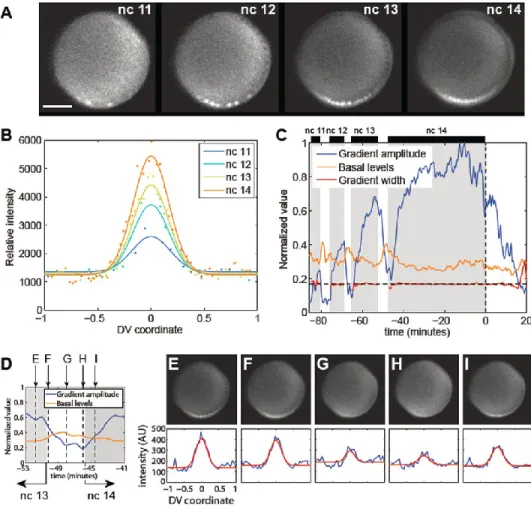
Another study reports active movement of Dorsal protein in and out of nuclei (DeLotto et al., 2007). Gradient amplitude (A), basal levels (B), and width (σ) parameters were determined using Gaussian fitting described in Materials and Methods, and each may vary over time (see Figure 3B and Equation 1 in Materials and Methods). Dorsal-Venus nuclear gradient measurements in three live embryos revealed similar results (see Figure S1).
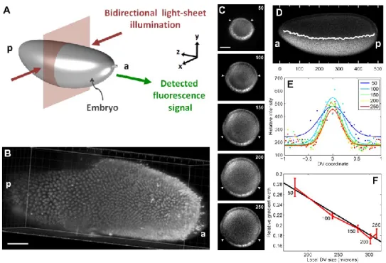
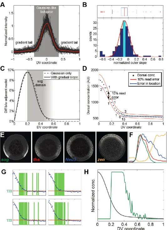
The mean slope of the gradient tail (normalized by the gradient amplitude) is the confidence interval; see histogram in Figure 6B). Live imaging of the Dorsal-Venus embryos was performed using two-photon scanning light-sheet microscopy (Truong et al., 2011).
INTRODUCTION
First, it involves using the entire secondary data set, rather than small sets of different points. Second, because it uses the entire data set, it is robust to noisy secondary data. Because of these advantages, we can be confident in our ability to detect very subtle phenotypes that are otherwise difficult to discern, either by eye or by comparison between sets of secondary data.
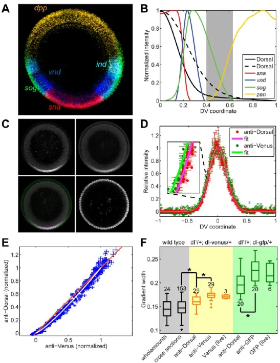
As a concrete example, we focus on the transcription factor Dorsal (dl), which functions as a morphogen in the early Drosophila embryo (rev. in Moussian and Roth, 2005). Dorsal can also act as a transcriptional repressor and in this function restrict the expression of some genes such as decapentaplegic (dpp) and zerknüllt (zen) to dorsal regions (rev. in Reeves and Stathopoulos, 2009; Stathopoulos and Levine, 2005). ). In this paper, we describe the steps in the image analysis protocol and provide details of the calculations involved in the data fitting procedures.
We demonstrate two cases where our analysis protocol has allowed us to detect subtle, but statistically significant, phenotypes in the dl patterning system. In the first case, we detect the slightly longer decay length in the nuclear gradient of a Venus-tagged version of dl compared to the nuclear gradient of wild-type dl (Reeves et al., 2012). The second case consists in measuring the subtle perturbation in the location of the vnd dorsal border in embryos that exhibit wider gradients.
We also present an example of image analysis in a different system from a cross section of a Drosophila embryo.
MATERIALS AND METHODS
- Collection, fixation and in situ hybridization of embryos
- Embryo manipulation
- Confocal imaging
- Image analysis
For the success of the image analysis, it is crucial to have only the desired embryo in the image, and no other fluorescent materials, such as other embryos or dust. The intensity of the image as a function of (the distance from the center of the image) is found for each slice in (Figure 2B). The assumed location of the boundary of the embryo is where the intensity drops rapidly (red dot in Figure 2B).
The next step is to detect average intensities around the periphery of the embryo, and is described briefly in (Reeves et al., 2012), and in more detail here. To accomplish this, the strip of nuclei is averaged in the radial (i.e., the apical-basal) direction to yield a one-dimensional representation of the nuclei (Figure 4C). Next, a watershed algorithm is used to determine the 1D locations of the cytoplasmic regions between nuclei.
Then, the pixels corresponding to each nucleus in the unrolled strip are mapped back to the original 2D image of the embryo (Figure 4D). Together with the data for the centroid of each nucleus, these measurements give us a relationship between nuclear protein intensity and location on the periphery of the embryo. Together with the data for the centroid of each nucleus, these measurements give us a relationship between intronic dot intensity and location on the periphery of the embryo.
First, the locations of the nuclei are merged into a minus one to one mesh with 300 points.
CALCULATION
Normalization with respect to nuclear intensity
We also assume that the concentration of the nuclear species is the same in each nucleus throughout the embryo, which means that the expression can simply be represented by a constant. Thus, this normalized intensity, , is simply proportional to the concentration, , up to an additive background constant. After normalizing each nuclear protein intensity to the corresponding nuclear stain intensity, the value is typically close to one.
Data fitting
Consider a canonical gene expression profile, ( ), with a peak located at , where is the coordinate along the DV axis of the embryo (Figure 6A). From these two parameters, we can calculate the dorsal and ventral limits of our measured gene expression profile. The canonical gene expression profile, ( ), has a dorsal and ventral border associated with it, defined as the location where the peak falls to half-maximal intensity (Figure 6A).
However, we report the results of the dorsal and ventral boundaries of gene expression as the average of the boundaries calculated from both sides, significance and. The two parameters and refer to the maximum intensity of the peak and the background levels of image intensity, respectively. Here, the terms and the radii represent the 68% confidence intervals on these parameters, and can be thought of as the size of one standard deviation.
One thing to note is that this fitting procedure requires that the ventral midline of the embryo has been previously identified. This can be done either manually (see example 3, section S1.8.7 in the supplementary material), by fitting another molecular species that allows clear identification of the midline (e.g., nuclear gradient dl; see section 3.2 .2), or through a rule-based procedure. Using this empirical model, the peak amplitude in the gradient dl is, the gradient.
The parameter σ will also be related to the width of the profile, but the strict definition of σ will be lost.
RESULTS
Expanded dl nuclear gradient in embryos carrying a copy of Venus-tagged dl The wildtype dl nuclear gradient conforms to a Gaussian-like decay with sloping
However, the secondary data obtained from our image analysis protocol shows that the gradient detected by anti-GFP is wider than that detected by anti-dl (Figure 8B,C). Using our empirical model of the dl gradient, we measured the width of these two gradients. This difference between these distributions in width across the set of 29 embryos is statistically significant, using the t-test for correlated samples (p-value < 10-6; Reeves et al., 2012).
We also found that the gradient detected by anti-dl in dl-venus embryos is broader than the dl-nuclear gradient in wild-type embryos. In summary, this implies that the magnitude of the actual spatial gradient of dl-Venus in the dl-venus embryos is wider than the gradient of endogenous dl (compare with ) in the same embryos. Because the anti-dl antibody will recognize both endogenous dl and dl-Venus, the anti-dl measurement in these embryos ( ) is an intermediate value.
Additionally, measurement of the dl-Venus gradient using anti-GFP is supported by measurements of Venus fluorescence in living dl-venus embryos ( Figure 8D ). The same trend is seen in embryos from mothers with a null allele of endogenous dl and a gfp-tagged copy of dl (hereafter referred to as dl-gfp embryos; see Figure 9). The width of the gradient as detected by anti-dl ( ) is not as wide as that detected by anti-GFP ( ), however both are wider than wild type.
Live studies of these embryos also show that the anti-GFP measurement is accurate (Figure 8D).
Shifted vnd dorsal border in embryos with expanded dl gradients
Quantifying gene expression profiles in other geometries: saggital sections of Drosophila embryos
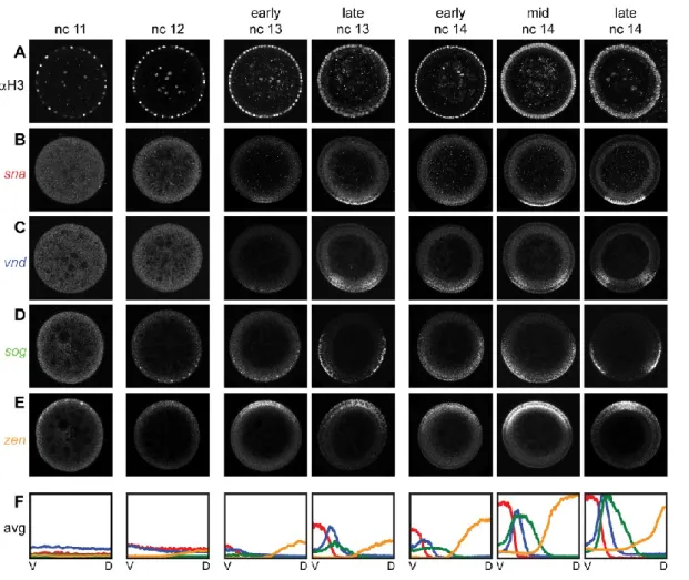
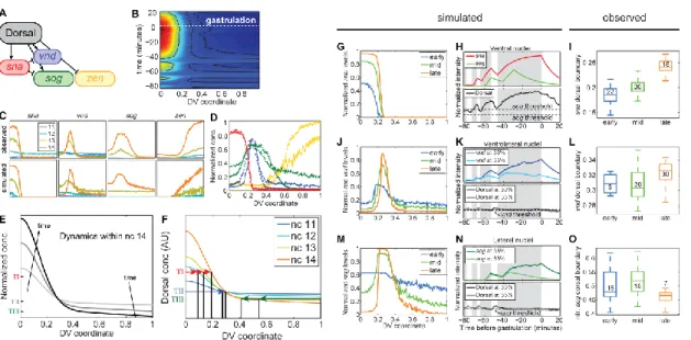
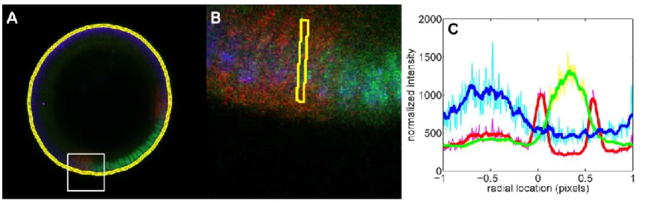
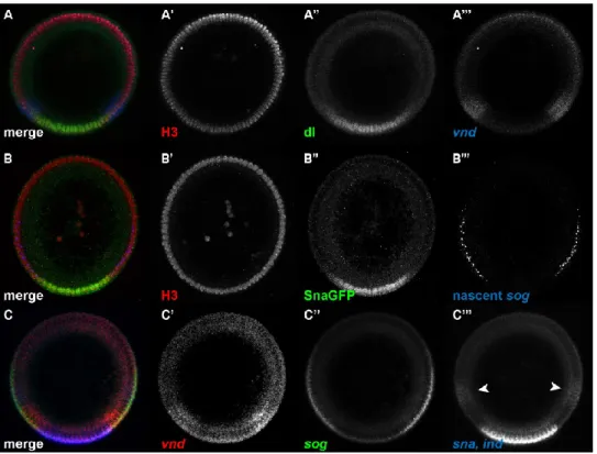
We selected embryos expressing a dominant form of the Toll receptor (Toll10B) present in an anterior-posterior gradient (see section 2 Materials and Methods; Huang et al., 1997). The endogenous, ventral-to-dorsal nuclear gradient of Dorsal is absent in these embryos, replaced instead by an anterior-posterior nuclear gradient of Dorsal. We hybridized these embryos with riboprobes against sna, vnd, sog, and ind (Figure 10A) and determined their gene expression profiles in the sliding window around the embryo periphery (Figure 10B; . Compare with Figure 3).
Apart from generating new canonical profiles for each gene, no program changes are required due to different spacings as a result of changing geometry. Note that both sna and ind occupy the same color channel; our peak fitting procedure can distinguish between two peaks (Figure 10C). This example demonstrates the program's ability to quantify profiles in different geometries and distinguish between two gene expression peaks in the same color channel.
DISCUSSION
Manual nuclear identification solves this issue (Reeves et al., 2012), but is not part of the code presented here. For each domain shown in (A), the points where it is determined to be the boundary of the embryo. The white square shows the part of the image shown in (B). B) Higher magnification of the area shown in (A).
Before centering the centerline, 0 is considered the bottommost point of the embryo in the image. The image shown in (A) averaged in the vertical direction to reveal a 1D representation of the nuclei. The blue and red solid curves are the fits of the canonical pattern to the measured right and left patterns, respectively.
The solid red and solid light green curves are the fits to the empirical model of the dl gradient (Equation 1). White curve: plot of the fit of anti-dl vs the fit of anti-Venus. Cyan and magenta circles are the right and left halves of the sna/ind plot in (B), respectively.
The blue and red solid curves are the fits of the canonical model to the measured models on the right and left sides, respectively.
Mesoderm spreading during Drosophila gastrulation
Supplementary Materials for Chapter II Chapter II
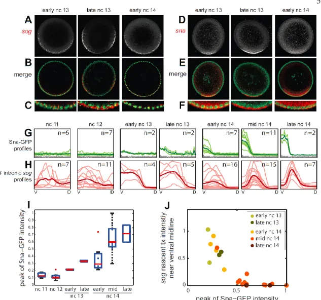
-Ventral gene expression in the Drosophila embryo reflects the dynamics and precision of the dorsal nuclear gradient. Characterization of the Dorsal gradient Simulations of gradient tail slopes Measuring gene expression profiles Analysis of intronic sog. Average of the three live Dorsal-Venus nuclear gradient time series Simulation of the Dorsal gradient.
-D) Plot of gradient amplitude, basal levels and gradient width (interphase only) of Dorsal-Venus from three separate live embryos. The gray curve at the bottom represents the background levels, which is the intensity of the Venus channel in a control embryo carrying only H2A-RFP. The 820 bp intronic sog probe used in this study starts at the beginning of the first intron (red bar).
Analyzes of additional embryos are shown in Figure 5G-J. Figure S4: Detection of gradient tail slope. Error bars indicate the standard error of pixel intensities in each kernel (also in B,D). The red curve is the possible non-uniformity in the intensity of the cores, based on real.
The peak of this curve is randomly placed with respect to the peak in the Dorsal gradient (i.e. the presumed ventral midline).