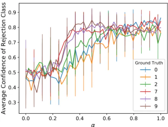
The RBF version of InceptionV3 is more robust than the regular model to all the attacks tested and also expresses a decrease in confidence to the conflicting images. 15 III.5 The deep RBF's rejection class confidence increases as the α value con-. trolling increases the opacity of the anomaly for the 6 classes targeted by the physical attack while decreasing the standard deviation of the confidence.
A Quick Overview of Security Threats Facing Deep Neural Networks
As for, a poisoned model can succumb to the attack while maintaining high confidence on clean data. Only recently it has been shown that a deep RBF can be successfully trained on MNIST dataset [19];.
Major Contributions
Outline
Section VI.1 summarizes the findings and describes potential areas of future work using deep RBFs.
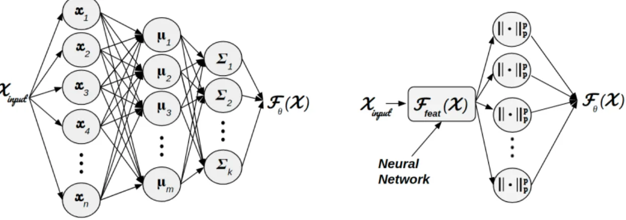
Deep RBF Network
Definition
Training a Deep RBF
Interpreting the Deep RBF Output
Related Research
For example, Deepxploreis is a white-box framework that first detects potential corner patches in the model by analyzing neuron coverage of the training decision and then produces patches for the problem [29]. Our work is most similar to outlier detection methods, which have previously relied on clustering of the training space [31] or higher Levelfeature space partitioning to detect outliers or regions of the network lacking sufficient training [32]. Autoencoder anomaly detectors have also been proposed, which rely on the latent space representation of the input to perform anomaly detection [33, 34].
Our intuition is that a deep RBF trained on a sparsely poisoned dataset will lower its confidence in the target (poisoned) label due to the presence of clean image features in the poisoned image allowing RBF deep to create a discriminating order of purity. and poisoned data.
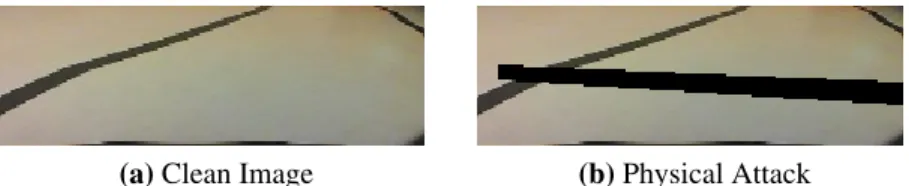
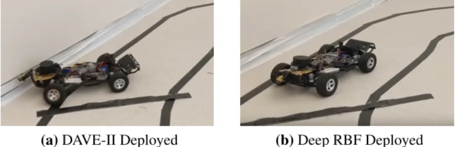
Black-Box Physical Attack Setup
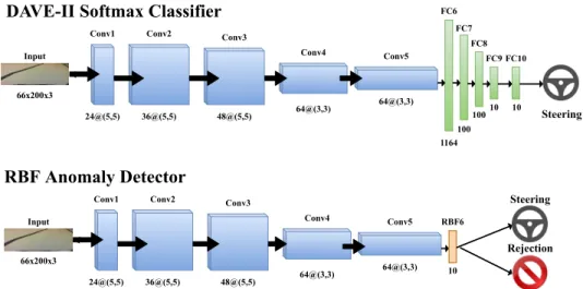
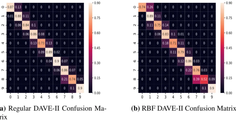
We denote a successful attack on the regular DAVE-II model and the deep RBF model based on the dangerous criteria defined below by a boolean statement. where fθ specifies which trained model is currently being attacked. The dangerous criteria are chosen because no fθ model violated the ˆyi>1±yi bound on the pure test data set when the rejection class was ignored for deep RBF as shown by the confusion matrices in Figure III.3. The criteria ensure that the deep RBF prediction is considered dangerous if the prediction is off by more than one true class and RBF fails to reject the class.
In the clean data, no model had a risky prediction, although deep RBF had a false-positive rejection rate of 0.25.
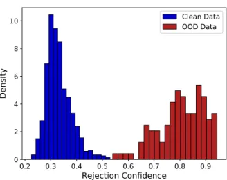
Offline Out-of-Distribution Detection Results
In the online attack, we use γ =0.6, which covers the end of the rejection class confidence for both the clean and OOD data (see Figure III.4). Without the rejection criteria, the deep RBF classifier would have predicted an unsafe situation 89% of the time due to the physical attack. In comparison to the pure test data, Figure III.4 shows how the deep RBF exhibited a significant shift (p<0.001) in the confidence of the rejection class for the physical attack data.
As the anomaly becomes more present in the clean image, the standard deviation of the confidence also decreases.
Online Out-of-Distribution Detection Results
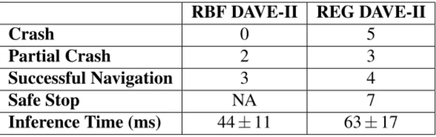
Because the DAVE-II model is an end-to-end black box DNN, we consider four scenarios to evaluate the results of the 12 trials. A collision is when DeepNNCar completely leaves the track; apartheid collision is when DeepNNCar partially leaves the track but recovers; successful navigation is when DeepNNCar does not leave the lane; and in the case of the deep RBF, a safe stop when the rejection class causes DeepNNCar to stop safely before the physical attack. It is typically assumed that the attacker has limited influence on the training procedure and access to a small, fixed portion of the data set.
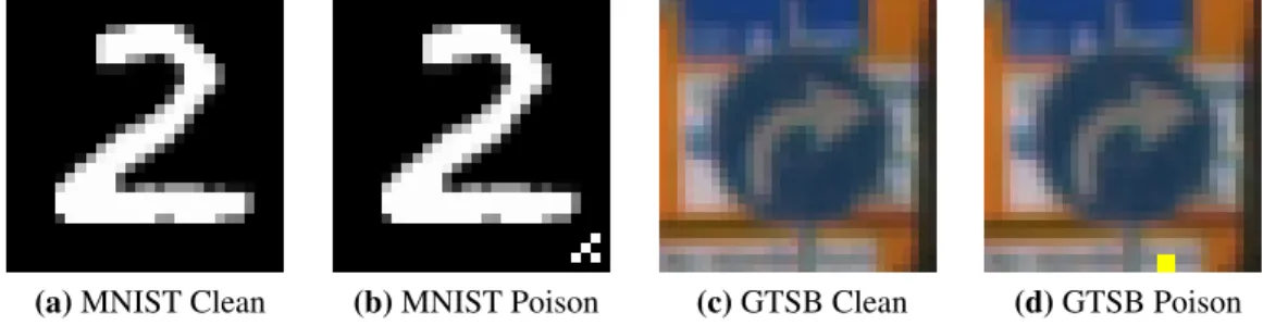
We adapt a popular pattern-key injection attack where the labels of the training dataset are changed each time the backdoor key is encoded into the training input, allowing an attacker to exploit the attack by encoding the backdoor key into the test instance [ 12] [ 13].
Data Poisoning Attack Setup
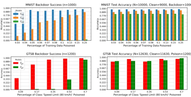
Data poisoning attacks modify the training procedure to allow the attacker to exploit the adversary's DNN. For the MNIST data poisoning attack, we train three CNN models fm1, fm2 and fm3. This is to explore the effects of the fully connected layer in a rolling tag attack.
Both models are trained on the poisoned dataset (n=39209) for 10 epochs and evaluated on 11430 clean test images and 1200 backdoors.
Explaining the Data Poisoning Results
This is likely due to a lack of architecture capacity and makes it unclear whether this was the reason fm3 did not succumb to the MNIST poisoning attack. In fact, fg1's poisoning success rate is greater than 30% after only 5% of the class data is poisoned, despite fg2 having better overall accuracy in that trial. We can also see that fg2 eventually succumbs to the poisoning attack, but requires more than 30% of the 80 km/h class data to be poisoned to only get a poisoning success rate approaching 30%.
However, the RBF layer must sacrifice the actual learned representation of the target class to encode the back-end logic which increases the error in clean data for both the target class and the base class.
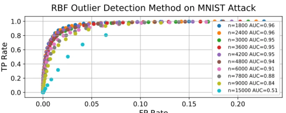
RBF Outlier Detection Method
In summary, the data poisoning results can be explained by comparing the effects of a high-dimensional dot product in the case of a regular classifier and the highly non-linear RBF operation that forces the deep RBF to learn strict, feature-based representations of the data. The area under the curve (AUC) score provides an overall measure of the performance of a binary classifier for different values of β. For the MNIST attack, the AUC is greater than 90% until the data poisoning exceeds 10% of the total training set (np=10000).
Second, a comparison of MNIST and GTSB RBF outlier detection cleaning reveals that as the accuracy of the detector increases on clean data, so does its ability to clean effectively.
Comparison of RBF Outlier Detection and AC Method
However, the RBF method begins to fail as the number of poisoned cases increases, while the performance of the AC method increases dramatically. In summary, the RBF outlier detection method is more effective in sparse poisoning conditions, while the AC method is more effective when a significant portion of the training dataset is poisoned. This is expected as the AC method requires a significant number of poisoned cases to consider them as a unique group, while our RBF outlier detection method requires a significant number of clean data to consider the poisoned cases as outliers.
Nevertheless, the ability to control β in the RBF outlier detection method makes it easy to adjust the number of true positives at the sacrifice of false positives, while it is less obvious how we can better target the AC method under rare poisoning conditions.
Adversarial Attack Setup
Adversarial attacks manipulate the input space by adding invisible non-random noise, typically using linear neural network gradient approximations to induce a high-confidence misprediction [10]. In this paper, adversarial attacks are created using the IBM Adversarial Robustness toolbox [43] which provides an API for performing FGSM, I-FGSM, Carlini & Wagner, Deepfool and PGD. We evaluate a non-trivial architecture to show that RBF units still increase robustness against adversarial white attacks despite using a model with sufficient capacity for realistic CPS tasks.
Experimentally, we found that for FGSM, I-FGSM and PGD, it is useful to adjust the parameters ε, ∆ε=0.0001, which control the added amount of interference or the change of interference (for iterative algorithms) to create a more realistic advertisement. sarial pictures.
Definition of Robustness
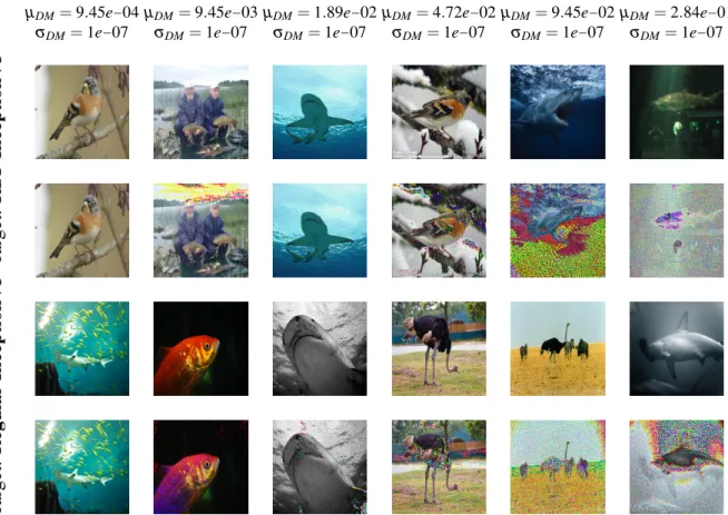
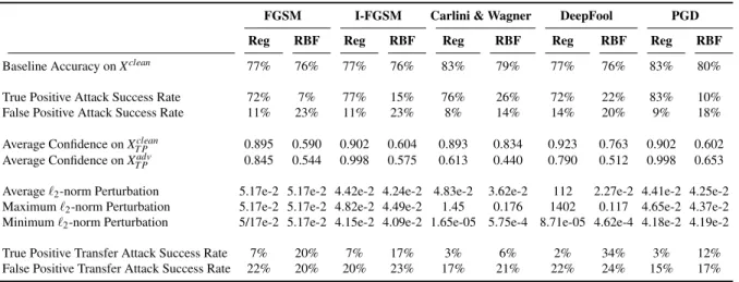
The regular InceptionV3 classifier and its RBF counterpart achieve an accuracy of 79.95% and 78.11% respectively on the clean test data (n=1950). The top row in each pair represents the clean image and the bottom row represents the conflicted image. Each column shows an example image of a batch (n=100) where the mean and standard deviation of the strain measure DM of the batch is recorded at the top of each column.
Using this formal definition of robustness, we can compare different models by analyzing the success rate of adversary attacks in relation to the amount of disruption added to Xi.
Evaluation of Adversarial Attacks
Results of Adversarial Analysis
Random images were selected to create conflicting batches (n=100) with different average distortion measures using FGSM to target the regular model and the RBF model. Third, the FGSM attack appears to be more effective in targeting the RBF model than injecting random noise; however, there is no significant difference (p>0.05). Second, adversarial algorithms are able to partially succeed by exploiting the linearity of the previous layers, which is why we see that an attack on the RBF network is more effective than a random noise attack, as effective as the transfer attack on the regular model, but less effective than the direct attack on the regular model.
This is because FGSM can partially exploit the linearity of the layers preceding the RBF layer.
Discussion and Future Work
However, the RBF outlier detection method has the added advantage of being easily tunable and with fewer hyperparameters. Therefore, future work should focus on using the RBF outlier detection method in a visual analysis tool to help assess potential poisoned samples and evaluate the effects of selecting various hyperparameters. Future work should focus on injecting RBF activations into intermediate layers to increase the robustness of the network.
Additionally, although we only investigated classification tasks, future work may find ways to feed RBF activations into segmentation, detection, and regression networks.
Conclusion
Clune, “Deep neural networks are easily fooled: high-confidence predictions for unrecognizable images,” inProceedings of the IEEE conference on computer vision and pattern recognition, pp. Manzagol, “Extracting and compiling robust features with denoising autoencoders,” inProceedings of the 25th International Conference on Machine Learning, pp. Jana, “Deeppxplore: Automated whitebox testing of deep learning systems,” inProceedings of the 26th Symposium on Operating Systems Principles, pp.
Easwaran, “Towards secure machine learning for cps: infer uncertainty from training data,” in Proceedings of the 10th ACM/IEEE International Conference on Cyber-Physical Systems, p.