Environmental Sustainability and Disaster Prevention – Fakultas Teknik Sipil dan Lingkungan

(1)

The Third Joint Seminar of Japan and Indonesia Environmental Sustainability and Disaster Prevention (3^rd ESDP-2015)

Institut Teknologi Bandung, Indonesia – November 25^th, 2015

1

MODELING OF WET DEPOSITION IN CHEMICAL TRANSPORT SIMULATION

Toshihiro Kitada

National Institute of Technology, Gifu College Japan

Email: [email protected] Presenter; † Corresponding author.

Abstract: Transport/chemistry/deposition model for atmospheric trace chemical species is now frequently used as an important tool to assess the effects of various human activities, such as fuel combustion and deforestation, on human health, eco-system, and climate. In the analysis of the serious release of radioactive species from the accident of Fukushima Daiichi Nuclear Power Plant in March, 2011, various models were also applied to estimate the amount of discharged radioactive materials and to understand observed spatial distributions (Sectional Committee on Nuclear Accident, Science Council of Japan, 2014[11]; hereafter abbreviated as SCNA). The SCNA report shows that results of some models and also ensemble average of the calculated results of all the participated models successfully captured main features of horizontal distribution of the accumulated deposition of 137Cs. However, it seems there are still by factors of 5 and 1/5 differences between observed and calculated results at the largest.

Thus in this paper I like to show our previous attempts on wet deposition in chemical transport simulation for reference to think about the phenomena. The chemical transport model is required to reproduce correctly mass balance of various chemical species in the atmosphere with keeping adequate accuracy for calculated concentration distributions of chemical species. For the purpose, one of the important problems is a reliable wet deposition modeling, and here, we introduce two types of methods of “cloud-resolving” and “non-cloud-resolving” modeling for the wet deposition of pollutants.

Keywords: Air pollution, transport modeling, wet deposition, cloud resolving/non-resolving

INTRODUCTION

Historically several models such as RADM[2] and STEM-II [1] included not only gas/aerosol phase chemistry but also aqueous phase chemistry in cloud/rain water in addition to the processes of advection, diffusion, wet deposition (mass transfer between aqueous and gas/aerosol phases), and dry deposition. Software of CMAQ (Community Multi-scale Air Quality model [3]) has been released by EPA for public use of a “comprehensive” model. These models are now frequently used by many people, and show their ability to successfully reproduce some features on atmospheric environment such as high ozone concentration episode by photochemical smog reactions. Figure 1 shows a model system for atmospheric trace chemical species. Meteorological model provides hydrometeors’ fields as well as flow, temperature, and eddy diffusivity to the comprehensive model for chemical species. Final target of the “comprehensive” model will be that the model can correctly reproduce mass balance of various chemical species in the atmosphere with keeping adequate accuracy for calculated concentration distributions of chemical species; in this situation life times of various primary and secondary pollutants should be correctly predicted. To do so many problems may be still remained. One of the important problems is reliable wet deposition prediction. There may be two types of attitudes for the modeling of the wet deposition; one considers trans-horizontal-grids transport of aqueous phase chemical species with use of partial differential equations for these species, and another one completes cloud processes within each vertical column, that is, a This Paper has been Presented at The 5th Environmental Technology and Management Conference (ETMC 2015)

(2)

2 simplified modeling.

In the following sections, we will introduce our previous attempts on these modeling techniques..

CLOUD-RESOLVING MODELING

Cloud-resolving modeling describes dynamics of chemical species in hydrometeors with unsteady partial differential equations, and allows the chemical species to cross grid cell boundary. It usually treats detailed mass transfer processes of chemical species among gas/aerosol and hydrometeor phases. Let us imagine the situation of the complex mass transfer taking place in the atmosphere. First, aerosol may serve as condensation nuclei to form cloud droplets. Then the cloud droplets either further grow with the processes such as accretion and auto-conversion to rain drop or with the Bergeron process to snow particle, or they may disappear by evaporation. These cloud processes can be summarized as Fig. 2 [4, 5, 10].

Associated with each cloud process shown in Fig. 2, inter-phase transfers of air pollutants such as SOx (SO2, and SO42-) and NO3- can occur among the phases of gas (aerosol), cloud

Figure 1. Comprehensive model of transport/transformation/deposition of atmospheric trace chemical species.

(3)

3

water, rain water, cloud ice, and snow. For example, mass transfer and transformation of SOx may be written as in Fig. 3. In addition, aqueous phase chemical reactions such as oxidation of SO2 (aq) in cloud and rain water take place as listed, for example, in Table 1 and 2.

Figure 2. Diagram of inter-hydrometeor-transfers of water substance of the cloud microphysics model after Rutledge and Hobbs, 1984 [4, 5, 10].

(4)

4

Figure 3. Schematic showing gas-hydrometeor inter-phase transfers of SOx [4, 8]. ✝The gas phase chemistry model includes the following reactions for SO42- production as main mechanism: SO2+OH→SO42- (lumped mechanism), SO2+RO2→SO42- (lumped mechanism), SO2→SO42- (oxidation reaction on the surface of aerosol particle). AbD, Absorption-Desorption; Acc, Accretion; Aut, Autoconversion; Ber, Bergeron process; BrD, Brownian diffusion; Col, Collection; Con, Conversion; EvR, Evaporation; ImS, Impaction scavenging; Mel, Melting; NuS, Nucleation scavenging; Oxi, Oxidation; Rim, Riming;

SuR, Sublimational Release.

(5)

5

Hence governing equations for chemical species in gas (and aerosol) and hydrometeors are summarized as follows:

For gas and aerosol phase species,

ij i i

i R S G

C t K

C       



 ¹ V C_i ~

 ^ , i = 1, 2, ……, I1 (1)

where Ci is the non-dimensional concentration of the ith chemical species in gas phase, ^ is the air density, Ri is the chemical reaction rate, Siis the non-flux-type emission source, and Gi^j is

Table 2. Aqueous phase chemical reactions [5].

10⁴

Table 1. Aqueous phase equilibrium reactions [5]

(6)

6

the mass transfer rate between gas and the jth hydrometeor phases; the rate consists of the relevant processes, for example, for SOx shown in Fig. 3.

For chemical species in hydrometeors,

 



 _j _i^j _k _i^j _i^j

j i i j j j i j j i j j

i j j

i R T G

z C V q z

q W C y

q v C x

q u C t

q

C  

 

 



 



 



 



 , i = I1+1, ….., I2 (2)

where Ci^j is the concentration of the ith chemical species in the jth hydrometeor, q_j is the water content of the jth hydrometeor, Wj wVj, Vj is the gravitational falling velocity of the jth hydrometeor such as rain, snow, and graupel, for which prescribed size distributions are assumed; for example, so-called Marshall-Palmer size distribution [9],

 jDjdDj

oj j

D N

N _,  exp^^ and

25 . 0













j oj

j jq

N



  for rain, snow, and graupel;

j

ND_, stands for the number density of droplets of the jth hydrometeor in the diameter range between Dj and Dj+dDj, and j is the density of the jth hydrometeor. Ri^jis the chemical reaction rate of the ith species in the jth hydrometeor, and _kT_i^j is the mass transfer rate of the ith chemical species between the jth and kth hydrometeors, the inter-phase mass transfer processes among hydrometeors are shown, for example, in Fig. 3; the term Ri^j is formed with the chemical reactions in Table 1 and 2.

APPLICATION OF CLOUD-RESOLVING MODELING: ACIDIC SNOW FORMATION OVER THE SEA OF JAPAN

In winter, cold air mass is accumulated over Siberia, and huge amounts of air pollutants, emitted from East Asian continental countries such as China and Korea, are also injected into the air mass. When this cold and pollutants-rich air mass flows out over the warmer Sea of Japan, thermal convection develops to form organized roll vortices aligned with main wind direction heading toward Japan. Hence the humid air mass, supplied with water vapor from the Sea of Japan, frequently brings heavy snow fall and also acidic deposition in the coastal area of Japan on the Japan Sea side. To analyze how and how much the acidic species are formed in the cloud streets associated with the roll vortices, our cloud-resolving model was used [5].

Figure 4 illustrates relative location of the East Asian countries, the Sea of Japan, and Japan, and also shows typical direction of the cold and polluted air mass movement and typical time required for the air mass’s crossing of the Japan Sea; as an example, approximate time of the passage is written in the figure. Figure 5 is the calculation domain idealized as two-dimensional situation.

(7)

7

Figures 6a,b show the calculated water content maps of cloud water and snow, respectively. They are the results after 12 hours’ advancement of the air mass over the Japan Sea.

Similarly, Figures 7a,b,c are the calculated pH and SO42- in the cloud water, and SO42- in the snow, respectively. Figure 7a suggests (1) the pH value of cloud water over the Japan Sea in winter can be around 4 or less, (2) the pH value is lower where the cloud water content is smaller; thus, pH is low at the edge of the cloud. The contour map of SO42- in Fig. 7b indicates (3) SO42- is trapped at the cloud base where upward air flow exists and (4) SO42- accumulates at the cloud top, in particular, in the interstitial air of the clouds. However, (5) SO42- in the snow phase is much larger than in the cloud phase as shown in Fig. 7c. Interestingly, the cloud and

Figure 5. Schematic diagram of the 2-D calculation domain for convective cloud streets over the Japan Sea in winter, where qv denotes water vapor mixing ratio, and θ the potential temperature [4, 5, 8].

Figure 4. Typical traveling course of the continental air mass moving over the Sea of Japan in winter; formation of cloud and formation of acidic species associated with the cloud were simulated along the course. The locations of the air mass at 0800, 1400, and 2000LST are indicated with thick solid arrows. The symbols from “A” to “H” represent observation points for acid deposition.

(8)

8

snow formation sometimes keeps pollutant concentration in the lower atmosphere rather high as suggested in Fig. 8, which compares vertical profiles of SO42- between D1 (with cloud and snow) and D0 (without them) cases; that is, in the cloud and snow case the cloud traps the pollutant and the snowfall returns the pollutant in the cloud again to the below-cloud level, and if the sublimation of the snow occurs, then the pollutant can be backed to gas and aerosol phase in the lower layer; of course, if there is no condition for the snow sublimation, then the pollutant in the snow will deposit onto the earth’s surface without raising atmospheric concentration.

NON CLOUD-RESOLVING MODELING

Non cloud–resolving modeling usually (1) does not use unsteady partial differential equation for chemical species in hydrometeor phases, (2) does not allow the pollutants in

0 1.6 3.2 km

Figure 8. Vertical profiles of calculated aerosol-SO42-: the cases of D0 (no-cloud) and D1 (cloud) at 2000LST along y=10.5 km [4, 5, 8].

Aerosol-SO42-

Height, z (km)

Horizontal distance, y (km)

(a) Cloud water (b) Snow

3

37

Figure 6. Vertical cross sections of calculated (a) cloud water, and (b) snow at 2000LST;

unit in g kg-air^-1 [4, 5].

(9)

9

hydrometeor phases to directly cross horizontal grid cell, and (3) is thus a simplified approach;

many of the comprehensive models such as RADM [2], STEM-II [1], and CMAQ [3] currently use this non cloud-resolving model.

In this section we will introduce our non cloud-resolving modeling and its application [4, 6]. If we use a spherical coordinate to describe transport/transformation equation for trace chemical species, governing equation can be written as follows:

I i

CX X R

E r r C

g y

E X y C

x CE X x C X

y CV X x CU X t

C X

i i i

i

i i

i

..., , 2 ,1 ,

cos cos

1 2

2 2

2   



 







 



 











 







 



 



 



 



 

 

 



 





 

(3)

wheredxrcosd, dyrd,  



PP_T



/ is the normalized pressure coordinate,

T

S P

P 

  , 

 _ 



W g z t V

z







    



 







  

 ,

Xi is the non-dimensional concentration of the i th chemical species, C and ρ are the air density in kmol m^-3 and kg m^-3, respectively, θ and φ are the latitude and longitude, r is the distance from the earth’s center, Ps and PT are the atmospheric pressure at the earth’s surface and top boundary, respectively, z is the altitude of σ surface, U, V, and W are the wind velocity for φ, θ, and z directions, respectively,  is the vertical velocity in σ coordinate, and R_i is the chemical reaction term. In Eq. (3), the last term on the right hand side stands for the wet deposition process; Λ is the scavenging coefficient due to cloud water, rain, and snow, and was derived for aerosol particle and gaseous species as follows (see for detail Kitada [4]; Kitada and Nishizawa [6]:

For wet deposition of SO42- particle by rain drop [4],

75 . 0 4

,_rain 6 10 _rP

p   ^ 

 in s^-1 ,

and for that by snow [12],

 

2 6 ,

10 6 . 3

t a s w

psnow V

P g





  ^



 in s^-1 ,

where P is the precipitation intensity in mmhr^-1,_r is the collection efficiency of aerosol particle by rain and was assumed to be 0.3~0.5, _s is the same but by snow and is summarized in Slinn [13], _wand _a are the density of water and air in kgm^-3, respectively, and Vt is the average settling velocity of snow flake in ms-1, and Vt 



10251log₁₀ dc



/100 is recommended [7].

For wet removal of gaseous species by rain, the following equation was derived (Kitada [4];

Kitada and Nishizawa [6]):

H P

SO² 3.6

 



 and  10^⁶RTH_eff_,_SO₂

where H is the height of the cloud top in m, R is the universal gas constant (=0.082

(10)

10

1

1 

 mol K atm

 ), T is the air temperature in K, and H_eff_,_SO₂is the inverse of the effective Henry’s law constant for SO2 in mol^¹atm^¹ (see [5] and [6] for detail), and β is an “equilibrium index” and represents the ratio of the real S(IV) concentration to the hypothetical equilibrium S(IV) concentration in rain water; and was determined with a series of numerical experiments in which concentrations of S(IV) etc. in rain drop falling through polluted atmosphere were calculated; β is 1 for SO2, 0.38x10^-8 for HNO3, and 0.055 for H2O2.

(11)

11

APPLICATION OF NON CLOUD-RESOLVING MODELING

The model described in section 3 was applied for pollutants transport in East Asia. Figure 9 shows, as an example of the results, the calculated total deposition of N- and S-compounds for 14 days [6].

Figure 9. Calculated total deposition (dry + wet) in BASE case: (a) N- and (b) S- compounds in mmol m^-2(14 day)^-1. The calculation was performed from 00GMT March 1 to 00GMT March 15, 1994. Contour lines are drawn for 0.1, 0.2, 0.5, 1.0, and 2.0 in mmol m^-2(14 day)^-1.

(12)

12 SUMMARY AND CONCLUSION

Two types of the modeling methods for the wet deposition processes, i.e., “cloud- resolving” and “non-cloud-resolving”, were introduced. Examples of their applications were also briefly described. For meso- and micro-scale phenomena such as the formation of acidic fog, the cloud-resolving approach described here should be further investigated. Also in Fukushima Nuclear Power Plant case, to consider transport equations of radioactive materials in cloud and rain phases directly may lead to better agreement with observation. A recent meeting on the modeling of atmospheric transport and deposition of radioactive nuclei in the Fukushima case may be referred in the web site [14].

REFERENCES

[1] Carmichael, G.R., Peters, L.K. and Kitada, T. (1986) A second generation model for regional-scale transport/chemistry/deposition, Atmos. Environ., 20, 173-188.

[2] Chang, J.S., Brost, R.A., Isaksen, I.S.A., Madronich, S., Middleton, P., Stockwell, W.R. and Walcek, C.J.

(1987) A three-dimensional Eulerlian acid deposition model, J. Geophys. Res., 92, 14681-14700.

[3] CMAQ (2003) EPA Web Site, http://www.epa.gov/asmdnerl/model3/

[4] Kitada, T. (1994) Modeling of transport/chemistry/deposition of acidic precipitation, Meteorological Research Notes (Kisho Kenkyu Notes), Meteorol. Soc. Japan, No. 182, 95-117 (in Japanese).

[5] Kitada, T. and Lee, P.C.S. (1993a,b) Numerical modeling of long-range transport of acidic species in association with meso-β-convective clouds across the Japan Sea resulting in acid snow over coastal Japan―I. Model description and qualitative verifications, Atmos. Environ., 27A, 1061-1076; II. Results and discussion, Atmos.

Environ., 27A, 1077-1090.

[6] Kitada, T. and Nishizawa, M. (1998) Modeling study of the long range transport of acidic pollutants over East Asia and the west Pacific Ocean –Sensitivity of acid deposition to scavenging model parameters and emission source distribution, Journal of Global Environment Eng., Japan Soc. Civil Eng., 4, 1-29.

[7] Knutson, E.O. and Stockham, J.D. (1976) Aerosol collection by snow and ice crystals. Atmos. Environ., 10, 395- 402.

[8] Lee, P.C.S. (1993) Numerical Modeling of Long Range Transport of Acidic Species Associated with Meso-β- convective Clouds Across the Japan Sea in Winter, PhD. dissertation, Toyohashi Univ. Technology, 246p.

[9] Marshall, J. S. and Palmer, W. McK. (1948) The distribution of raindrops with size, J. Met., .5, 165-166.

[10] Rutledge, S. A. and Hobbs, P. V. (1984) The mesoscale and microscale structure and organization of clouds and precipitation in midlatitude cyclones. XII: a diagnostic model studying of precipitation development in narrow cloud frontal rainbands, J. Atmos. Sci., 41, 2949-2972.

[11] Sectional Committee on Nuclear Accident, Science Council of Japan (2014) A Review of the Model Comparison of Transportation and Deposition of Radioactive Materials Released to the Environment as a Result of the Tokyo Electric Power Company’s Fukushima Daiichi Nuclear Power Plant Accident, 103p.

[12] Slinn, W.G.N. (1974) Dry deposition and resuspension of aerosol particles – a new look at some old problems.

In Atmosphere-Surface Exchange of Particulate and Gaseous Pollutants, R.J. Engelmann and G.A. Sehmel (ed.), 1-40, NTIS, Springfield, Virginia.

[13] Slinn, W.G.N. (1977) Some approximations for the wet and dry removal of particles and gases from the atmosphere, Water, Air, and Soil Pollution, 7, 513-543.

(13)

13

[14] International workshop on dispersion and deposition modeling for nuclear accident releases -Transfer of science from academic to operational models- (2015)

http://venus.iis.u-tokyo.ac.jp/english/workshop/newE.htm

(14)

Bandung Institut Teknologi, Indonesia – November 25^th, 2015

15

EMISSION REDUCTION FROM IMPLEMENTATION OF BUS RAPID TRANSIT CORRIDOR 13th IN JAKARTA

Lailatus Siami¹, Asep Sofyan^2*,†, and Russ Bona Frazila³

1,2Environmental Engineering Department, Institut Teknologi Bandung, Jl. Ganesha No. 10, Bandung, Indonesia.

Email: [email protected]

3 Civil Engineering Department, Institut Teknologi Bandung, Jl. Ganesha No. 10, Bandung, Indonesia

* Presenter; † Corresponding author.

Abstracts: Green transport nowadays become important concern related to emission reduction. This is also become one of policy brief in Jakarta Macro Transportation (JTM) plan. Busway or so-called BRT as one of reliable mass tranportation in Jakarta has been developed for 12 corridor. 13^th corridor is planned as elevated with length 14.6 km typed 2 lanes 2 way. Are this scenario will be significantly affect for emission reduction? This main question will be figured out in this research. Eventually, emission of transportation sector in Indonesia reached almost 200 Gg/year up to 2012. In the research, road networking model is used for representing actual condition of complex urban road in Jakarta. By the result of road assignment, will be estimated the traffic volume every road. Hence, Emission load calculated by bottom – up emission inventory and carried out from road segmentation. Afterwards, emission will be mapped out by spatial distribution resolution 1 km x 1 km that reveals emission reduction due to development of busway 13^th is 9% of all emission, respectively. This sufficiently high rate of emission reduction due to fuel shift from fossil fuel to gas considered.

Keywords: Busway corridor 13^th, Road networking model, Emission Inventory, Load Emission

INTRODUCTION

The transportation sector is contributes around 23% of GHG emissions overseas (Li et al., 2010). In fact, this sector is the largest source of pollution of the atmosphere contributing to global warming (Progiou and Ziomas, 2011). Road transport contributed to the increase in emissions of air pollutants and cause environmental and health problems depends on the type and concentration of pollutants (Souza et al., 2013).

Jakarta, the capital city of Indonesia, keep becomes the largest center of urbanization which means mobility level of people and goods would higher constantly. In addition, with urban sprawl of the city will enforce people in suburb (Bodetabek) to do activity in the heart of Jakarta and daily moving in and to Jakarta. Traffic congestion has become usual pattern.

Car-oriented development is still the prevalent paradigm of urban development in the developing countries that triggers from exponential growth of private cars in emerging economies. The most widely adopted strategy on mass transportation is BRT development. BRT is a public transport concept that allows high-capacity buses to operate at a rapid speed with some priorities through an integrated system including dedicated lanes, stations, and technologies and advanced branding (United Nations Centre for Regional Development, 2014).

In Jakarta itself, traffic management conduct by Jakarta Macro Transportation (JTM) plan since 1985. It comprised by three main policies in mass transportation development, traffic restriction, and road capacity development. In line with these, DKI Jakarta Act No.1 of 2012

(15)

16

about Spatial Plan 2030, Article 22 paragraph (2) states that efficient road transportation will be realized if the target of 60% of the population using public transport and increase the average speed - the road network average a minimum of 35 km/h.

Regarding with emissions reduction, the existing literature has investigated the individual impacts of bus service improvements mostly. Yet, only few studies assessed the combined effects of various strategies on transit bus emissions (Alam et al., 2014).

The main objective of this research is to know the effect busway 13^th corridor in reduct the emission load in 2017. The study will covers CO, NOx, PM10 and VOC from car, motorcycle, bus, minibus and truck. The method used in this study is road network model and adapted Emission inventory from EMEP / European Environment Agency in 2013. The emissions inventory is the basis of air quality modeling and analysis and also to understand the shape and the transport of pollutants and the reference to pollution control (Fu, et al 2013). However, many factors that affect vehicle emissions and large amounts of data will be needed in the inventory of emissions from vehicles. So, it is arduous to develop an accurate inventory of emissions for major cities (Wang et al, 2008).

Description of the study corridor

DKI Jakarta is capital city of Indonesia lied on 6^o12’ south latitude and 106^o48’ east longitude with the width 662.33 km² (BPS, 2012). The study location includes all public roads and toll (Figure 1). Type modes of transportation in Jakarta are divided into mass transit and private vehicles. For mass transport is dominated by minibus, bajaj and busway. While, private vehicles consisting of cars and motorcycles.

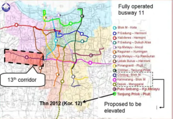
Nowadays, the number of busway is already in operation reached 12 corridors (Figure 2).

And the number of passengers in 2012 reached 304,799 passengers/day or 111,251,869 passengers annualy. As for the plan of development with elevated busway are on 13, 14 and 15 corridors whereas the line 13^th connecting Ciledug - Blok M. Corridors 14^th connecting Kalimalang - Block M. And corridor 15^th connecting Depok – Manggarai.

METHODOLOGY Calculation

In this study, the calculation of vehicles number is use road network model. As for input are OD (Origin - Destination) matrix and road networking data (Arifin, 2012) of Jabodetabek in 2012 (SATURN, 2013). In the network model, the area is divided into several zones of travel.

Each zone is represented by 1 zone center (centroid) connected to the road network through the centroid connector. Here, the road network in Jakarta road network is divided into some 42 zones (see Table 2).

(16)

17

Table 1. Number and Zone of Jakarta Road System

No Zone No Zone

211 Gambir 241 Tebet

212 Sawah Besar 242 Setiabudi

213 Kemayoran 243 Mampang Prapatan

214 Senen 244 Pasar Minggu

215 Johar Baru 245 Kebayoran Baru 216 Menteng 246 Kebayoran Lama 217 Tanah Abang 247 Cilandak

218 Cempaka Putih 248 Pancoran 222 Penjaringan 249 Jagakarsa 223 Tanjung Priok 251 Matraman

224 Koja 252 Pulo Gadung

225 Cilincing 253 Jatinegara 226 Pademangan 254 Kramat Jati 227 Kelapa Gading 255 Pasar Rebo 231 Kalideres 256 Cakung 232 Grogol Petamburan 257 Duren Sawit 233 Tamansari 258 Makasar 234 Tambora 259 Ciracas 235 Kembangan 261 Cipayung 236 Cengkareng

237 Palmerah 238 Kebon Jeruk

OD Matrix to be assigned in Jabodetabek road network data is as follows (see Table 3).

Table 2. In part OD Matrix 2012 Zone 211 212 …. 510 511

211 0 405 …. 2 14981

212 410 0 …. 2 5464

…… …… ….. …. …… ……

510 2 2 …. 0

511 16102 5778 …. 235 379468

(17)

18

The vehicles number passing each segment of road in the city represent as vehicles volume in units pcu/h is converted into the number of vehicles with passenger car equivalence (Department of Public Works, 1997). Emissions inventory calculations performed road segments when the vehicle working and using the following equation (EMEP / European Environment Agency, 2013):

E i, k,T = Nk× LA,T × e i, k (1)

Ei, k, T is pollutant emission of i[g] at time T. Nk is vehicle typed k. L a,T is length roadof a [km] at time T. And e i, k is emission factor [g/km] for pollutan i, for vehicle typed k, at time T. Emission factor showed by Table 4 below.

Table 3. Summary of Emission Factor

No. Pollutan Vehicle Typed Emission Factor (g/km)

1. CO Car 37.3

Motorcycle 14.7

Bus 5.71

Minibus 2.71

Truck 1.85

2. NOx Car 1.8336

Motorcycle 0.0576

Bus 15.84

Minibus 8.989

Truck 4.183

3. VOC Car 2.77

Motorcycle 8.18

Bus 1.99

Minibus 0.706

Truck 1.07

4. PM10 Car 0.0022

Motorcycle 0.176

Bus 0.909

Minibus 0.479

Truck 0.333

Source: EMEP- Corinair, 2013

Transportation demand was forecasted for 2017 using the main transportation network in place in 2012. The transport networks in BAU scenarios in 2012 and 2017 are assumed to be the

(18)

19

same. The 2017 BAU scenario assumes that elevated busway 13^th corridor would be implemented in 2017. The scenarios with the corresponding assumptions on transport network and enforced policies are summarized in Table 5.

Table 4. Summary of Emission Factor Scenario Transport network and

enforced policies

Baseline 2012 Transportation demand + No action

BAU 2017 2017 Transportation demand + No action

Busway 2017

2017 Transportation demand + Elevated Busway 13^th Corridor development

Figure 1. Study area of DKI Jakarta (PU Cipta Karya, 2012)

Policy scenario were developed based on the mass transportation typed Bus Rapid Transit/Busway, this is based on a comparison of the cost of the various types of mass transit (see Table 1).

(19)

20

Table 5 Characteristics of Mass Transportation (Velocity,Construction Cost, Capacity)

Source: ITDP in transportation department in figures 2012, 2012

Mass transportation with the most efficient velocity, capacity passanger and total investment is bus rapid transit (BRT/busway). Some developing Asian cities consider BRT in their public transport planning because of its advantages of lower investment cost and flexible implementation over rail systems. Moreover, BRT is recommended that would shift private vehicle users to a transport sector which emits lower CO2 (Satiennam et al, 2015).

Figure 2.Busway corridor which has been operating in the city of Jakarta in 2012 (Transportation Department in figures, 2012)

On previous study (Ernst, 2006) showed that the possibility of shiftment from private transportation to buses by 14%. In the scenario, elevated busway to be implementated is corridor 13^th. The length of the corridor 13^th is 14.6 for a type of application 2x1 lanes (2 lanes 2 way).

RESULTS AND DISCUSSION Traffic Volume

OD Matrix to be assigned to the Jabodetabek road network data for baseline is shown in

(20)

21 Table 6 below.

Table 6 In part Result of Baseline Zone 211 212 …. 510 511

211 0 405 …. 2 14981

212 410 0 …. 2 5464

…… …… ….. …. …… ……

510 2 2 …. 0

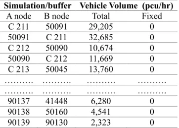
511 16102 5778 …. 235 379468 So the vehicles volume on the road traffic Jakarta as follows.

Table 7 In part Result of Baseline Vehicle Volume Simulation/buffer Vehicle Volume (pcu/hr)

A node B node Total Fixed

C 211 50091 29,205 0

50091 C 211 32,685 0

C 212 50090 10,674 0

50090 C 212 11,669 0

C 213 50045 13,760 0

………. ………. ………. ……….

90137 41448 6,280 0

90138 50160 4,541 0

90139 90130 2,323 0

Details proportion of passing vehicles on the main road and highway can be seen in Figure 5. The roads with the densest volumes are on the road Ciputat Raya. The number of cars, motorcycles, buses, minibuses, and trucks respectively - helped as many as 10,132; 49,076; 280;

407 and 650 units a day. The number of cars and trucks at most dominating motorway Gatot Subroto respectively - also 7823 and 4477 units per day.

(21)

22

Figure 3. Mode Share based on typed in Jakarta by 2012

The proportion of vehicles that dominate the toll road in Jakarta is a car, whereas on a main road motorcycles dominate. This is the main cause of congestion (Ferdinansyah, 2009).

The level of preference for private vehicles in Jakarta is quite high due to social status, security and comfort of the rider. Lacks of public transport services also trigger the use of private vehicles (Dissanayake and Morikawa, 2010).

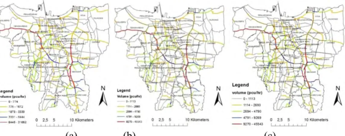
At baseline, where a scenario have not be applicable in 2012. The volume of vehicles on each road follows the path of a primary arterial road (Figure 4). In West Jakarta, the heavy volume of vehicles are in Cengkareng sub-district is on the road Daan amounted to 31,662 pcu/h (passenger car unit/hour). This is due to the high number of trips from the town Tangerang to Jakarta and vice versa (Sunggiardi, 2009). In addition, compared to other major roads in Jakarta, Daan Mogot road is one of the arterial roads at speeds below 10 km/h (Putranto, 2010). Activities dominant land use in the surrounding streets is in the form of services trade industry, and offices.

In South Jakarta, the heavy volume of vehicles are in Kebayoran Lama sub-district is on the road Ciputat Raya amounted to 23,992 pcu/h. The basic capacity of 4,950 pcu/h and per direction basis capacity of 5,560 pcu/h. Triggers number of vehicle volume is due to the use of the main road to the mobility of vehicle and to South Tangerang. In Ciputat there are also several small terminal, as in Jombang market, Bintaro market and Serpong market. Certainly, this will increase the number of vehicles passing on Ciputat Raya road. In East Jakarta, in Kramat Jati district heavy volume of vehicles crossing located on the May. Jend. Sutoyo street of 7,137 pcu/h. Several roads with heavy volumes estimated road network model are the road with high- frequency congestion. This is in line with the data traffic jam-prone areas in Jakarta.

Highway has a volume of most solid vehicles are toll roads Gatot Subroto in Central

(22)

23

Jakarta area Tanah Abang subdistrict with a volume of 16,470 pcu/h. Volume ratio and capacity on the road is around 0.91. This means that the road almost reached the degree of saturation. Toll road in East Jakarta with heavy volume is Jagorawi and the junction with the volume of vehicles Cawang 7,182 pcu/ h and 6,831 pcu/h. One treatment to reduce the density of vehicles in Jakarta is the modal shifts vehicle. Modal shifts of vehicles from cars and motorcycles allows changes to the ratio of VOC/NOx in the atmosphere (Nugroho, 2010).

The spread of the volume of vehicles on the scenario BAU 2017 did not undergo significant changes as well as Scenario of busway 2017. West Jakarta areas with high vehicle volume remained at Daan Mogot Street.

(a) (b) (c)

Figure 4. (a) Traffic Volume each segment in Jakarta by 2012. (b) Traffic Volume each segment in Jakarta by 2017. (c) Traffic Volume each segment in Jakarta based on busway 13^th scenario by

2017 Load Emission

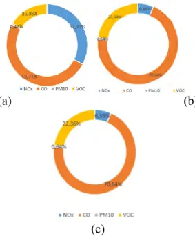
As a whole, baseline emission inventory on road segmentation in Jakarta by 2012 resulted 148,343 Gg/yr for NOx; CO as 229,953 Gg/yr; PM10 as 2,089 Gg/yr. and VOC emission as 72.867 Gg/yr. CO plays the largest contribution as 50,73% of all pollutants and NOx as 32,73% as the second largest (Figure 5a). Meanwhile BAU scenario 2017 resulted emission load of NOx as 29,687Gg/yr; CO as 330,748 Gg/yr; PM10 as 3,003 Gg/yr and VOC as 104,807 Gg/yr (Figure 5b). After Busway corridor 13^th applied, NOx as 29,651.47Gg/yr; PM10 as 2,991.55Gg/yr and VOC as 104,269.76 Gg/yr. CO still play as the largest emission for 329,377.52 Gg/yr and reached 72.48% of all pollutant typed (Figure 5c).

As we can see in Figure 6 above, the BAU Scenario resulted the largest emission load of NOx pollutant is laid on toll roads, toll roads i.e. IR. Wiyoto Wiyono with emissions amounting to 5,820.25 Gg/year. The highest NOx pollutants emissions on the main road, is located on the road of Ciputat Raya with emissions by 530.35 Gg/year. For NOx Emissions are highest on the motorway, although on a main road of vehicles is more varied.

(23)

24

(a) (b)

(c)

Figure 5. Emission Share of : (a) Baseline scenario in 2012. (b) BAU 2017 Scenario (c) Busway Corridor 13^th in 2017

This is due to the number of vehicles of trucks that travel the highway more than the number of vehicles traveling on the main road. In addition, the length of the road on toll roads with the highest emission is longer than the main road. Emission load of CO highs along the Jakarta-Cikampek toll road of 1,695.94 Gg/year. On the main road, the largest emissions load of CO is on the road Ciputat Raya amounted to 1,279.58 Gg/year. Meanwhile, the highest CO emission load is on the highway, this is due to the number of cars and trucks more in that way.

The largest PM10 emission load laid on toll roads, toll roads is located in IR. Wiyoto Wiyono with emissions amounted to 48.02 Gg/year. Emissions of the pollutants PM10 highest on the main road, is located on the road of Ciputat Raya with emissions by 10.82 Gg/year. On the highest emissions PM10 emissions are on the highway, although on a main road kind of vehicles is more varied. This is due to the number of vehicles of the same trucks that travel the highway more than the number of vehicles traveling on the main road. In addition, the length of the road on toll roads with the largest emission is longer than the main road. The highest VOC pollutants emissions load on the main street, namely in roads Ciputat Raya with emissions by 499.94 Gg/year. VOC emission load is in toll roads located in IR. Wiyoto Wiyono with emissions amounted to 430.28 Gg/year.

(24)

25

a) NOx (b) CO (c) PM10 (d) VOC

Figure 6. Emission Load Based on Type of Pollutant: Baseline in 2012 (up). BAU Scenario in 2017 (middle). Busway Corridor 13^th Scenario in 2017 (bottom).

In Figure 6 Middle can be seen, the emission load of each segment road in 2017 in DKI Jakarta. In General, the pattern of load emissions BAU scenario 2017 unchanged and only the values of the quantity of emissions are increasing at each toll road. When compared to scenarios Do – Nothing in 2012, pollutants NOx and VOC decline. While the pollutants CO and PM10, the shares of load emissions are fixed.

In Figure 6 below can be seen, the emission load of each segment road in Jakarta. VOC

(25)

26

pollutants Pattern is almost the same with NOx emissions burden, of which the highest are on the roads in and around Cawang Panjaitan. While the pattern of CO pollutant almost the same with those of PM10, where the highest emission is around toll road Cawang and Letjen. S.

Parman.

Table 8 Comparison of scenario result cenario Traffic

Volume (smp/jam)

NOx CO

(Gg/yr) PM10

(Gg/yr) VOC (Gg/yr) (Gg/yr)

BAU 2017 2,006 29 330 3 104.81 Scen. 3

Busway 2,002 25 326 2.43 103.06 Emission load

reduction (%) 13% 1% 19% 2%

CONCLUSION

Emission inventory on road segmentation in Jakarta by 2012 resulted 148,343 Gg/yr for NOx; CO as 229,953 Gg/yr; PM10 as 2,089 Gg/yr. and VOC as 72.867 Gg/yr. CO plays the largest contribution as 50.73% of all pollutants and NOx as 32.73% as the second largest.

However the largest emission load located in other lane and it is resulted that emission load reduction from Busway 13^th corridor operation is unsignificant with the rate 9%, repectively. In addition, the lane of this corridor is shorter compare than others. It is needs a further study to understand fully how much the exact emission load reduction of mode shitment to busway that illustrate CNG as fuel in combination with operational changes that lead to further improves emission reductions. To such degree emission reduction on busway depending on their operations, technology, age and passenger loading that eventually transit buses could be as polluting as private cars on a per passenger basis (Lau et al., 2012).

ACKNOWLEDGEMENTS

Research described in this article was partially supported by Research described in this article was partially supported by Hibah Kerjasama Luar Negeri dan Publikasi Internasional Direktorat Jenderal Pendidikan Tinggi (DIKTI) Indonesia and PEER USAID Cycle 3.

REFERENCES

Alvinsyah Z.A. Impact on the existing corridor due to implementation of new public transport corridor (case Study:

Jakarta BRT systems). The Eastern Asia Society for Transportation Studies 2005; 6: 467 – 479

Alam A, Diab E, El-Geneidy A.M, Hatzopoulou M, A simulation of transit bus emissions along an urban corridor:

Evaluating changes under various service improvement strategies. Transportation Research Part D 2014; 31:

(26)

27

189–198

Arifin Z.N. 2012. Route Choice Modeling Based On Gps Tracking Data: The Case Of Jakarta. Dissertation Badan Pusat Statistik (BPS), 2011. Jakarta in figure 2011. Jakarta.

Both AF, Westerdahl D, Fruin S, Haryanto B, Marshall JD. Exposure to Carbon Monoxide, Fine Particle Mass, and Ultrafine Particle Number in Jakarta, Indonesia: Effect of Commute Mode. Science of the Total Environment 2013; 443: 965–972.

Departemen Pekerjaan Umum, 1997. Manual Kapasitas Jalan Indonesia (MKJI), Direktorat Jenderal Bina Marga, Indonesia.Dinas Perhubungan Provinsi DKI Jakarta, 2012. Dinas Perhubungan Dalam Angka Tahun 2012.

Jakarta

Dissanayake D, Morikawa T. Investigating household vehicle ownership, mode choice and trip sharing decisions using a combined revealed preference/stated preference Nested Logit model: case study in Bangkok Metropolitan Region. Journal of Transport Geography 2010; 18: 402–410

European Environment Agency, 2013. EMEP/EEA air pollutant emission inventory guidebook 2013. Technical Guidance to Prepare National Emission Inventories EEA Technical Report No 12/2013. ISSN 1725-2237.

Ferdiansyah R. Kemungkinan Peralihan Penggunaan Moda Angkutan Pribadi ke Moda Angkutan Umum Perjalanan Depok – Jakarta, 2009; 20: 3

Han, S.S. Managing Motorization in Sustainable Transport Planning: The Singapore Experience. Journal of Transport Geography 2010; 18: 314–321

J.P. Ernst, Initiating Bus Rapid Transit in Jakarta, Indonesia, J. Transp. Res. Board 1903 (2006) 20–26.

Fu X, Wang S, Zhao B, Xing J, Cheng Z, Huan L, Jiming H, Emission inventory of primary pollutants and chemical speciation in 2010 for the Yangtze River Delta region, China. Atmospheric Environment 2013; 70: 39–50 Lau J., Hatzopoulou M., Wahba M.M., Miller E.J., 2012. Integrated multimodel evaluation of transit bus emissions

in Toronto, Canada. Transportation Research Record 2216, 1e9.

Li, Q., Xiaomeng, C., Cui, X., Tang, L., Li, Z., Liu, C., 2010. A road segment based vehicle emission model for real- time traffic GHG estimation. Paper presented at The Transportation Research Board 90th Annual Meeting, WashingGg, D.C.

Liu, WT, Chen SP, Chang CC, Yang, CFO, Liao, WC, Su, YC, Wu, YC, Wang, CH, Wang, JL, Assessment of Carbon Monoxide (CO) Adjusted Non-Methane Hydrocarbon (NMHC) Emissions of a Motor Fleet - A long Tunnel Study. Atmospheric Environment 2014; 89: 403–414

Nugroho S.B., Fujiwara A., Zhang J. The influence of BRT on The Ambient PM10 Concentration at Roadside Sites of Trans Jakarta Corridors. Procedia Environmental Sciences 2010; 2: 914–924

Progiou AG, Ziomas IC. Road traffic emissions impact on air quality of the Greater Athens Area based on a 20 year emissions inventory. Science of the Total Environment 2011; 1(7): 410-411

Putranto, L.S., 2010. Evaluation of Space Mean Speeds Of Road Links Surronding New Developments in Jakarta.

The Seventh Asia Pacific Conference on Transportation and the Environment. 3 – 5 June 2010 SATURN – Simulation Assignment of Traffic in Urban Road network Manual – version 11.2 2013

Susilo YO, Joewono TB, Santosa W, Parikesit D. 2007. A Reflection of Motorization and Public Transport in Jakarta Metropolitan Area

Satiennam T., Jaensirisak S., Satiennama W., Detdamrong S., 2015. Potential for modal shift by passenger car and motorcycle users towards Bus Rapid Transit (BRT) in an Asian developing city.

http://dx.doi.org/10.1016/j.iatssr. 2015.03.002 (accessed 05.01.15).

Sunggiardi R, Putranto LS, Motorcycle Potential Problems In Jakarta. Jurnal Transportasi 2009; 9 (2): 117-126 Souza C.D.R, Silva S.D, Silva M.A.V, D’Agosto M.A, Barboza A.P, Inventory of conventional air pollutants

emissions from road transportation for the state of Rio de Janeiro. Energy Policy 2013; 53: 125–135

United Nations Centre for Regional Development, 2014. Next Generation Sustainable Transport Solutions in the Context of post-2015 Development Era

Wang H, Chen C, Huang C, Fu L, On-road vehicle emission inventory and its uncertainty analysis for Shanghai, China. Science of the total environment 2008; 398: 60–67

(27)

28

Widodo CE, Kidokoro T, Implementing Transit-Oriented Development (TOD) in A Developing City: Residents’

Perception on TOD in Jakarta, Indonesia AESOP 26^th Annual Congress. 11-15 July 2012. METU, Ankara

(28)

29

ESTIMATION OF TOTAL CARBON EMISSION FROM FOREST FIRES: CASE STUDY OF BORNEO ISLAND

Arno Adi Kuntoro^1,*,†Ade Wahyu², Hendri³:

1Faculty of Civil and Environmental Engineering, Institut Teknologi Bandung, Indonesia Email: [email protected]

2Ministry of Environment and Forestry of Indonesia Email: [email protected]

3Universitas Papua, Indonesia [email protected]

* Presenter; † Corresponding author.

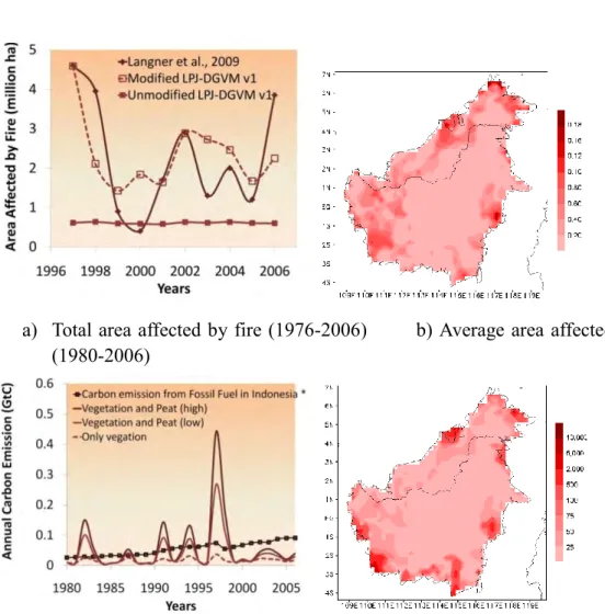
Abstract: The availability of combustible materials and their flammability are important aspects in forest fires studies, especially to predict the total carbon emission to the atmosphere. From point of view of earth system modeling, Dynamic Global Vegetation Model (DGVM) provides most of the basic computations for simulating the interactions between terrestrial ecosystem and the atmosphere, including carbon accumulation in vegetation bodies, litter and soil/peat, by considering the effect of climate conditions and its variability. In this study, a modified Lund Potsdam Jena Dynamic Global Vegetation Model (LPJ-DGVM) for application in tropical area is used to simulate the total amount of carbon emitted to the atmosphere in Borneo Island from 1980 to 2006. Simulation results show that the annual average carbon emission from forest fire in Borneo Island is 0.02 to 0.06 GtC/y, with the highest emission during 1997-1998 El-Niño event, which is about 0.05 GtC if only considering the burned of aboveground vegetation, to about 0.62 GtC by also considering the burned of peat layer.

Keywords: DGVM, forest fire, carbon emission, Borneo

INTRODUCTION

Tropical forests together with tropical peatlands are one of largest carbon storage in the terrestrial ecosystem. With average carbon stock per hectare about 157.1 t/ha, the total carbon stored in Asia and South East Asia was about 44.5GtC, in which about 31%was located within Indonesian territory [1]. The total areas of tropical peatlands were estimated about 38 million ha which mostly located in Southeast Asia.

Total peat carbon stored in this region was about 50.4GtC, with more than 90% was located in peatlands area in Indonesian territory [2]. In general, tropical forests and tropical peatlands act as a carbon sink.About 30% of Indonesian land territory is located in Borneo. Most area of this island was covered by rainforest. However, rapid land cover changes since the early 1970s has reduced its forest cover to about 71% in 1980s with further decrease up to 54% in 2000s [3]. Many studies suggest that large scale deforestation and forest fire might contributes to more CO2 emission to the atmosphere such those occurred during an extreme El-Niño in 1997-1998 which was followed by a large forest fire in Borneo Island [4],[5].

Forest fires can be analyzed from three aspects: combustible materials, their flammability and fire sources. This study is focused in the analysis of the availability of combustible materials, which is closely related to the estimation of total carbon pool in vegetation, litter and soil/peat and their flammability. Fire sources in human induced landscapes are quiet complex to be modeled. Such analysis should include various factors such as demography, distance of disturbed area to the forest boundary, road, etc., which is mostly beyond the capability of the current DGVM.

Many studies focused on field investigation and direct measurement, for example:[4],