EVIDENCE ON MONETARY POLICY TRANSMISSION DURING TRANQUIL AND TURBULENT PERIODS*

(1)

EVIDENCE ON MONETARY POLICY TRANSMISSION DURING TRANQUIL AND TURBULENT PERIODS*

Chioma Peace Nwosu**, Afees A. Salisu***, Margaret Johnson Hilili****, Izuchukwu Ifeanyi Okafor*****, Izuchukwu Oji-Okoro******, Idis Adediran*******

**Research Department, Central Bank of Nigeria, Abuja, Nigeria. Email: cpnwosu@cbn.gov.ng

***Department for Management of Science and Technology Development, Ton Duc Thang University, Ho Chi Minh City, Vietnam ; Faculty of Business Administration, Ton Duc Thang University, Ho Chi

Minh City, Vietnam; Centre for Econometric & Allied Research, University of Ibadan, Ibadan, Nigeria.

Email: afees.adebare.salisu@tdtu.edu.vn

****Research Department, Central Bank of Nigeria, Abuja, Nigeria. Email: mjhilili@cbn.gov.ng

*****Research Department, Central Bank of Nigeria, Abuja, Nigeria. Email: iiokafor@cbn.gov.ng

******Research Department, Central Bank of Nigeria, Abuja, Nigeria. Email: ioji-okoro@cbn.gov.ngd

*******Centre for Econometric & Allied Research, University of Ibadan, Ibadan, Nigeria.

This paper evaluates monetary policy transmission in both tranquil and turbulent periods for Mexico, Indonesia, Nigeria, and Turkey. Using a structural vector autoregressive model, we find that the effect of structural shocks from supply, demand, and financial sources tend to fizzle out faster for Nigeria and Mexico compared to Indonesia and Turkey. Another important finding is that while monetary authorities in Indonesia and Turkey are more responsive to inflation those in Mexico and Nigeria are more influenced by the exchange rate. We also observe differences in the conduct of monetary policy between the tranquil and turbulent periods.

Article history:

Received : July 23, 2019 Revised : September 23, 2019 Accepted : September 26, 2019 Available online : October 15, 2019 https://doi.org/ 10.21098/bemp.v22i3.1111

Keywords: Monetary policy transmission; Structural Vector Autoregressive model;

MINT countries; Global financial crisis.

JEL Classification: E44; G21.

ABSTRACT

* The authors thank the anonymous reviewers and the managing editor – Professor Paresh Kumar Narayan for their useful comments. The technical support received from the econometric workshops of the Central Bank of Nigeria is graciously acknowledged.

(2)

I. INTRODUCTION

The mandate of most central banks, particularly in emerging economies, still revolves around the maintenance of macroeconomic stability (Ngan, 2018; Binici et al., 2019; Egea and Hierro, 2019). Hence, an interesting area of research is the study of the direction and effectiveness of central banks’ monetary policy on prices and the real economy (Yagihashi, 2011; Ascarya, 2012). Among monetary policy transmission channels, the interest rate channel that links the financial and real sectors stands out as a major transmission route in these types of economies (see Ascarya, 2012 for empirical evidence on Indonesia and Binici et al., 2019 for empirical findings on Turkey). This route can be informed by the Taylor rule widely adapted to describe the behavior of central banks, since it accounts for inflation and output gap in setting policy rates (Taylor, 1993, 1999).

This study is therefore motivated to explore the interest rate channel of monetary policy transmission in Mexico, Indonesia, Nigeria, and Turkey, the MINT countries. These are emerging economies that either target inflation directly or indirectly via monetary aggregates (Beju and Ciupac-Ulici, 2015; Binici et al., 2019). Further, these economies have a pronounced interest rate channel, since central banks look to macroeconomic stability to drive investment (Wulandari, 2012; Papadamou et al., 2015). As a second contribution, we augment the Taylor rule to account for the role of the exchange rate, especially since the central banks in these economies intervene in the foreign exchange markets and have been shown to react to exchange rate, inflationary pressure, and output fluctuations in setting policy rates (Hutabarat, 2011; Chen et al., 2017; Froyen and Guender, 2017;

Ngan, 2018).¹

Our third contribution revolves around conducting these analyses for calm and turbulent episodes as determined by the Global Financial Crisis (GFC).

This is justified by the following. One, a new direction in the finance literature suggests rethinking the practice of monetary policy, given the realities such as the GFC (Mishkin, 2017). Two, evidence suggests that the macroeconomic effect of monetary policy differs considerably across these periods (e.g., Jannsen et al., 2015; Egea and Hierro, 2019). For the empirical analysis, we construct a structural vector autoregression model with strict exogenous variables (i.e. SVAR-X model) based on the augmented Taylor rule for each of the MINT countries. The SVAR-X model incorporates output, inflation, the exchange rate, and the interest rate as endogenous variables and accounts for strictly exogenous (“X”) global factors (i.e., the global oil prices and the global interest rate) that influence the financial markets.

In the final analyses, we clearly distinguish between the operation of monetary policy in these countries before and after the GFC. We also show that, although inflation in Indonesia and Turkey, which have adopted inflation targeting, exhibits a greater influence on the interest rate, monetary policy responds more to exchange rates in Mexico and Nigeria, although the importance of the level of economic activity has been growing in recent times in Nigeria.

1 Froyen and Guender (2017) provide empirical evidence showing that the exchange rate should be included in the Taylor rule, especially in economies where maintenance of exchange rate stability is a policy concern.

(3)

Following the motivation for this study, the remainder of the paper is organized as follows. Section II discusses the data and methodology. Section III discusses the results. Section IV checks the robustness of the results. Section V concludes the study.

II. METHODOLOGY AND DATA

We construct a structural VAR-X model with four endogenous variables for the interest rate channel of monetary policy transmission.² We formerly argued that the interest rate channel is theoretically implied in the Taylor rule of monetary policy.

In this framework, central banks take account of the level of economic activity and prices in their objective functions while setting their policy rates.³ Thus, to reflect the international macroeconomy, the ensuing empirical model incorporates output growth, inflation, the exchange rate, and the interest rate as endogenous variables (Taylor, 2001). Our motivation also implies that the monetary policy transmission mechanism is sensitive to structural shifts, such as the effects of the GFC, as well as global financial market fluctuations. Hence, we account for global oil prices and the global (US) interest rate in the interest rate equation. Thus, we justify a distinct analysis for the periods before and after the GFC and account for other structural changes posed by seasonal effects in the data.

We first specify the following standard VAR model as the baseline for the SVAR model:

where is a 4×1 vector of endogenous variables (growth rate of industrial output, inflation, log differences in the exchange rate, and changes in the nominal interest rate); is a matrix of contemporaneous effects; is a 4×1 vector of constants; is a 4×4 matrix of coefficients of lagged series for all ; is a vector of disturbances or structural innovation, serially uncorrelated, with a mean of zero; and p is the optimal lag, obtained using the Schwartz Information Criterion (SIC). The variables are transformed so as to circumvent nonstationarity in their level series.

Since the analysis of the structural VAR requires that the model be identified, we impose restrictions that satisfy the condition and a recursive approach. The study assumes a simple recursive structure of the model to identify structural shocks. The recursive restrictions derive from the intuition that:

• The interest rate does not have an immediate impact on the output gap.

• There is no contemporaneous relation between current interest rates and prices (inflation and exchange rate).

• The exchange rate does not have a direct impact on aggregate demand; in other words, there is no contemporaneous relation between the exchange rate and output.

2 The work is limited to the interest rate channel for brevity, and the analyses can therefore be replicated for other channels for potential generalization of the research findings.

3 Other channels of monetary policy transmission (e.g., the credit channel, the balance sheet channel, the asset price channel) have been noted, and strong motivation has been established for the interest rate channel.

(1)

(4)

• There is an interest rate rule (i.e., the Taylor rule) that states that central banks take into account current output growth and inflation in setting monetary policy rates.

• Central banks adopt an active stabilizing role in the foreign exchange markets.

From the foregoing, the matrix of contemporaneous effect ( ) is defined in Table 1. The standard SVAR model described in the analysis is augmented, based on the motivation, by some inherent effects (seasonal effects and structural changes) in the data sets, and the reconstructed model is described as an SVAR-X model. We demonstrate that including these effects in the analysis of the SVAR model can offer useful insights for policy decision purposes.

Table 1.

Restrictions on the Matrix

This table shows the recursive restrictions imposed on the matrix of contemporaneous effects. g_t, π_t, r_t and Δi represent industrial production growth, inflation, exchange rate returns and changes in interest rate, respectively.

Endogenous Variable Contemporaneous Variable

* 0 0 0

1 * 0 0

1 1 * 0

1 1 1 *

To estimate the standard SVAR model, we specify the reduced-form of equation (1) as

where and , with constants

suppressed for notational convenience. Having justified the recursive restrictions theoretically with the Taylor rule, we see the reduced-form residuals could follow a Cholesky decomposition-type orthogonalization. Thus, the matrix of initial impulse responses can be constructed as follows:

The shocks in the SVAR system are called the supply shock ( ) emanating from the output, demand shock ( ) is reflected in the general price level, financial shocks ( ) are transmitted via the exchange rate, and interest rate shock ( ) arises from monetary policy actions. In addition to the Taylor rule, the intuition for the (2)

(3)

(5)

absence of contemporaneous effects from the output or the price on the interest rate consists of the operational rigidities in the production process that create a lag between policy pronouncements and production. On the other hand, demand and supply shocks will evoke unanticipated policy responses from the monetary policy authority to remedy their long-term consequences on the economy.

The paper employs monthly data series for the Industrial Production Index (IPI), the Consumer Price Index (CPI), the Nominal Effective Exchange Rate (NEER), and the Interest Rate (INTR) covering the period from January 2000 to December 2018 for all the MINT countries, except Nigeria, where quarterly data spanning 2000Q1 to 2018Q4 were employed. The data for the other MINT countries were sourced from the International Financial Statistics database, and the data for Nigeria were sourced from the National Bureau of Statistics and the Central Bank of Nigeria databases. The data for the global factors, namely, the oil prices and US interest rates, were obtained from the Federal Reserve database.

III. RESULTS AND DISCUSSION

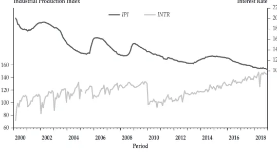
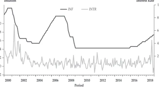
We attempt to briefly describe the variables of interest in Table 2 and Figures 1 through 3. In the data description, all four MINT countries record average interest rates sufficiently larger than that of the United States (1.95%), with 7.28% for Mexico, 14.02% for Indonesia, 18.17% for Nigeria, and the lowest, 4.81%, for Turkey.

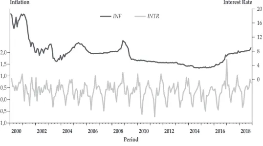
Notably, average inflation appears to be the highest in Nigeria (2.99%), where the rate of interest is also the highest, although the reverse cannot be inferred. On the other hand, the IPIs and the nominal effective exchange rates of the countries appear to be close. Figures 1 to 3 show that the variables are associated with the interest rate over time. Evaluation of the time series properties reveals that they are all stationary in the level expressed (for details of the transformation of the series, see the notes for Table 2). These findings are exhaustive, in that the results of both the conventional augmented Dickey–Fuller tests and the generalized autoregressive conditional heteroskedasticity-based Narayan–Liu unit root tests corroborate each other.

Table 2.

Preliminary Tests

The variables INT, IPI, INF NEER, US_INT, WTI and BRENT denote domestic interest rate, industrial production index, inflation, nominal effective exchange rate, US interest rate, West Texas Intermediate and Brent oil prices.

Inflation is computed as log in differences of consumer prices (CPI) as follows: 100^*Δlog(CPI). The descriptive statistics of the series (mean, standard deviation (SD) and Jarque-Bera (JB) statistics) are computed on the level forms of the series. The unit root tests (Augmented Dickey Fuller [ADF] and Narayan & Liu [NL] (2015) tests) are conducted on the growth rate of IPI and returns series of NEER, WTI and BRENT, the differenced series of INTR and US_INTR computed as: Δ(INTR) and Δ(US_INTR). Superscripts a & b represent 1% and 5% significance levels, respectively.

Finally, * and ^ represent the inclusion or exclusion of trend component in the underlying unit root test equation, respectively.

Variables

Description

Mexico Indonesia

Mean SD JB ADF NL Mean SD JB ADF NL

INTR 7.278 3.33 160.4^a -12.9^ -15.8* 14.02 2.56 23.0^a -5.5^ -9.1*

IPI 102.4 6.50 11.6^a -8.24^ -27.4^ 118.2 13.0 1.57 -21.4^ -43.2*

INF 0.365 0.34 12.8^a -10.4* -12.9^ 0.544 0.74 27947^a -12.3* -16.1*

NEER 106.8 23.6 6.6^b -11.9^ -14.3^ 98.19 18.5 9.46 -11.1^ -12.6*

(6)

Figure 1. Trends in Industrial Production Index and Interest Rate in the MINT Countries, 2000-2018

The plots are arranged in the order of MINT countries from the top left to down right. The MINT acronym denotes Mexico, Indonesia, Nigeria and Turkey.

IPI INTR

85 90 95 100 105 110 115

0 4 8 12 16 20

2000 2002 2004 2006 2008 2010 2012 2014 2016 2018

Trends in Industrial Production Index and Interest Rate in Mexico, 2000M1 to 2018M12

Industrial Production Index Interest Rate

Period Table 2.

Preliminary Tests (Continued)

Nigeria Turkey

Mean SD JB ADF NL Mean SD JB ADF NL

INTR 18.17 2.56 38.3^a -9.2^ -19.9^ 4.81 1.90 46.4^a -6.42* -75.1^

IPI 107.6 10.6 6.33^b -10.3^ -362* 106.2 34.6 12.5^a -11.5^ -22.4*

INF 2.993 2.26 15.4^a -8.2* -7.6* 1.107 1.36 903^a -3.12^ -10.8*

NEER 109.4 32.9 1.80 -8.0^ -8.9* 105.0 57.3 529^a -10.0^ -12.7^

Global factors

Mean SD JB ADF NL

US_INT 1.952 1.96 37.7^a -10.2* -18.1^

WTI 62.16 26.7 11.3^a -11.1* -10.9*

BRENT 64.73 30.6 15.3^a -12.0* -11.1^

(7)

Figure 1. Trends in Industrial Production Index and Interest Rate in the MINT Countries, 2000-2018 (Continued)

Trends in Industrial Production Index and Interest Rate in Indonesia, 2000M1 to 2018M12

60 80 100 120 140

160 10

12 14 16 18 20 22

2000 2002 2004 2006 2008 2010 2012 2014 2016 2018

IPI INTR

Period

Trends in Industrial Production Index and Interest Rate in Nigeria, 2000Q1 to 2018Q4

IPI INTR

80 90 100 110 120 130

12 16 20 24 28

2000 2002 2004 2006 2008 2010 2012 2014 2016 2018

Period

(8)

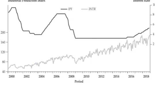
Figure 1. Trends in Industrial Production Index and Interest Rate in the MINT Countries, 2000-2018 (Continued)

Trends in Industrial Production Index and Interest Rate in Turkey, 2000M1 to 2018M12

IPI INTR

40 80 120 160 200

2 4 6 8 10

2000 2002 2004 2006 2008 2010 2012 2014 2016 2018

Period

Figure 2. Trends in Inflation and Interest Rate in the MINT Countries, 2000-2018

Trends in Inﬂation and Interest Rate in Mexico, 2000M1 to 2018M12

INF INTR

-1,0 -0,5 0,0 0,5 1,0 1,5 2,0

0 4 8 12 16 20

2000 2002 2004 2006 2008 2010 2012 2014 2016 2018

Inﬂation Interest Rate

Period

(9)

Figure 2. Trends in Inflation and Interest Rate in the MINT Countries, 2000-2018 (Continued)

Trends in Inﬂation and Interest Rate in Indonesia, 2000M1 to 2018M12

INF INTR

-2 0 2 4 6 8 10

10 12 14 16 18 20 22

2000 2002 2004 2006 2008 2010 2012 2014 2016 2018

Period

Trends in Inﬂation and Interest Rate in Nigeria, 2000Q1 to 2018Q4

INF INTR

-8 -4 0 4 8 12

12 16 20 24 28

2000 2002 2004 2006 2008 2010 2012 2014 2016 2018

Period

(10)

Figure 2. Trends in Inflation and Interest Rate in the MINT Countries, 2000-2018 (Continued)

Trends in Inﬂation and Interest Rate in Turkey, 2000M1 to 2018M12

INF INTR

-2 0 2 4 6 8 10

2 4 6 8 10

2000 2002 2004 2006 2008 2010 2012 2014 2016 2018

Period

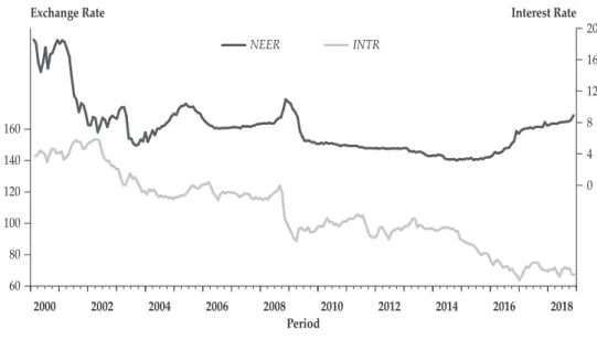
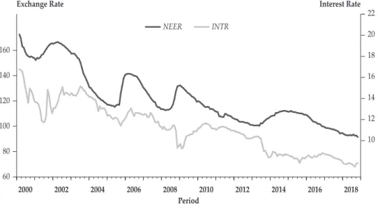
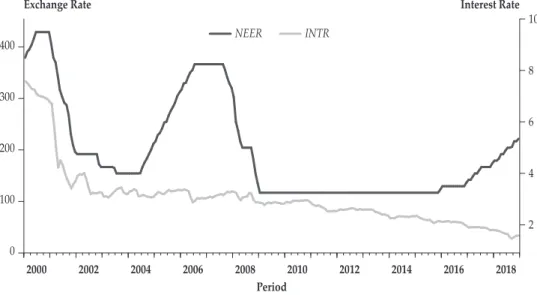
Figure 3. Trends in Exchange Rate and Interest Rate in the MINT Countries, 2000-2018

Trends in Exchange Rate and Interest Rate in Mexico, 2000M1 to 2018M12

NEER INTR

60 80 100 120 140 160

0 4 8 12 16 20

2000 2002 2004 2006 2008 2010 2012 2014 2016 2018

Exchange Rate Interest Rate

Period

(11)

Figure 3. Trends in Exchange Rate and Interest Rate in the MINT Countries, 2000-2018 (Contined)

Trends in Exchange Rate and Interest Rate in Indonesia, 2000M1 to 2018M12

60 80 100 120 140 160

10 12 14 16 18 20 22

2000 2002 2004 2006 2008 2010 2012 2014 2016 2018

NEER INTR

Period

Trends in Exchange Rate and Interest Rate in Nigeria, 2000Q1 to 2018Q4

40 80 120 160 200

12 16 20 24 28

2000 2002 2004 2006 2008 2010 2012 2014 2016 2018

NEER INTR

Period

(12)

As argued previously, we explore an SVAR-X model that accounts for seasonal effects, with distinct analyses for the periods before and after the GFC.

The underlying optimal VAR model for the SVAR-X is determined using the information provided by the SIC for selection among competing models. The SIC selects an optimal lag of one for all the models across the four countries. The resulting model is evaluated for the coefficients of the contemporaneous effects, impulse responses, and variance decomposition functions. In the analysis of the contemporaneous effects (see Table 3), the relevant coefficients are C3, C5, and C6, representing the immediate effects of the IPI and inflation and exchange rates, respectively, on the interest rate. The impulse response graphs are constructed such that the responses lie within +2 standard deviations. The forecast horizons for the shock analysis are set at 10, but the monetary policy variance decompositions for periods 1, 5, and 10 are selected for a summary. The results are highlighted as follows.

Figure 3. Trends in Exchange Rate and Interest Rate in the MINT Countries, 2000-2018 (Contined)

Trends in Exchange Rate and Interest Rate in Turkey, 2000M1 to 2018M12

NEER INTR

0 100 200 300 400

2 4 6 8 10

2000 2002 2004 2006 2008 2010 2012 2014 2016 2018

Period

(13)

Pre GFCPost GFCFull Sample C1C2C3C4C5C6C1C2C3C4C5C6C1C2C3C4C5C6 Panel A: Mexico 0.018 (0.01)0.124 (0.08) 0.049 (0.04) 0.317 (0.77) -0.23 (0.345) 0.251 (0.046) -0.01 (0.01) -0.02 (0.12) -0.016 (0.013)

0.427 (1.01)

0.13 (0.11) 0.012 (0.009) 0.0003 (0.007)0.051 (0.07)0.008 (0.020) 0.552 (0.645) 0.058 (0.173)

0.071a (0.017) Panel B: Indonesia

0.02 (0.01) 0.050 (0.05) 0.003 (0.002)

0.27 (0.40)

-0.02 (0.02) 0.003 (0.005)

0.02b (0.01)

0.05 (0.03) 0.001 (0.002) 0.092 (0.41) -0.03 (0.02) 0.008c (0.004)0.016b (0.008)0.048 (0.03) 0.002 (0.002)

0.158 (0.255)

-0.01 (0.013) 0.002 (0.003)

Panel C: Nigeria

0.022 (0.14) -0.18 (0.17)

0.093c (0.055)

0.253 (0.21) -0.07 (0.071)

0.047 (0.059)

0.03 (0.13) 1.99a (0.62)-0.34a (0.056)0.540 (0.72) 0.04 (0.05) 0.017 (0.012)-0.029 (0.097) 0.270 (0.27) -0.008 (0.048) 0.132 (0.327)-0.071 (0.056) 0.046 (0.020)

Panel D: Turkey 0.032c (0.017)

-0.08 (0.08) 0.003b (0.001)2.33a (0.52) -0.01 (0.012) -0.002 (0.002)

0.03b (0.01)

0.02 (0.04) 0.001 (0.001)

1.88a (0.36)

0.004 (0.01) -0.005b (0.002)0.024b (0.010) -0.02 (0.043) 0.001 (0.001) 1.928a (0.280)0.009 (0.008)-0.003b (0.001)

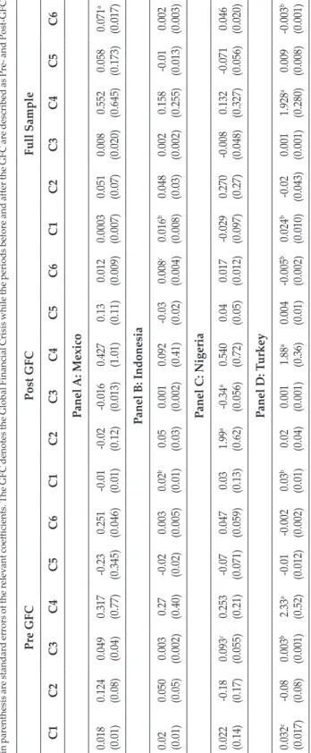
Table 3. Results for Contemporaneous Effects In this table, C1, C2 and C3 represent the contemporaneous effects of IPI on inflation, exchange rate and interest rate, respectively. C4 and C5 are the contemporaneous effects of inflation on exchange rate and interest rate, and C6 is the contemporaneous effect of exchange rate on interest rate. Superscripts a & b represent 1% and 5% significance levels, respectively. Values in parenthesis are standard errors of the relevant coefficients. The GFC denotes the Global Financial Crisis while the periods before and after the GFC are described as Pre- and Post-GFC.

(14)

For all the countries, the supply shock (i.e., the C3 coefficient) exerts positive effects on the interest rate in the calm period (i.e., pre-GFC). The results are consistent with economic theory, although the coefficient proves to be rather nonsignificant, except in Turkey. However, a sign reversal takes place for Mexico and Nigeria, whereas the weight of the negative impacts is greater in Nigeria, affecting the full sample. Hence, although a coefficient variation exists across periods for Mexico and Nigeria, it is absent for Turkey and Indonesia. A plausible reason for its absence in Turkey and Indonesia is that, in turbulent times, the monetary authorities tend to use unconventional measures that might not reflect a priori expectations. We also observe contrasting results for the two data samples in terms of the contemporaneous effect of inflation on the interest rate (i.e., the C5 coefficient) for Mexico, Nigeria, and Turkey, but not Indonesia. Given the empirical results, the monetary policy authorities in Mexico, Nigeria, and Turkey tend to respond to the prevailing macroeconomic dynamics, as evidenced in the contrasting signs between the pre- and post- GFC periods. However, such a contrast between the pre- and post GFC periods is not observed for the immediate impact of financial shock (the C6 coefficient) on monetary policy across the countries.

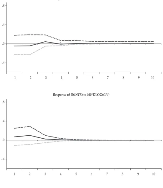
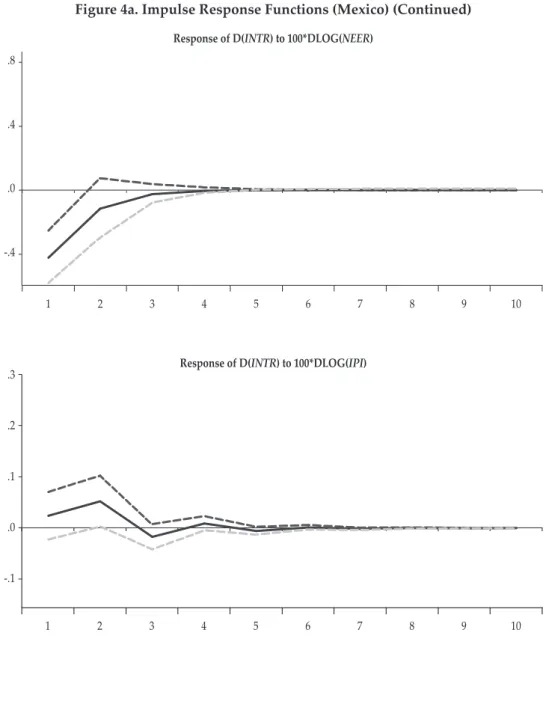
Beyond the contemporaneous relations, we employ impulse response functions to show the responses of the interest rate to the three macroeconomic shocks, that is, supply, demand, and financial shocks. By design, impulse response functions also determine whether the effects of these shocks are transient or permanent. The impulse response functions in Figures 4a to 4d are arranged in rows and columns such that the rows show the results of the analysis for the pre-GFC period, the post-GFC period, and the full sample, while the columns shows the responses of the interest rate to supply, demand, and financial shocks respectively. Hence, the figure in the ith row and jth column represents the response of monetary policy to the jth macroeconomic shock for the ith data sample.

The analysis shows that all three shocks are transient in the system, although it took different time horizons for this to be achieved in each country. The transitory nature of the shocks is shown in Figures 4a to 4d by the blue line in between the +2 standard deviations (upper and lower dotted red lines) being tangential to the horizontal line at the specified period. Just as the findings revealed under the contemporaneous effects, the plots show evidence of contrasting relations, shown by the impulse response functions for pre- and post-GFC (in support of Jannsen et al., 2015; Mishkin, 2017; Egea and Hierro, 2019). However, the clear exception is Indonesia, for which no such effect is observed across the data samples or across the macroeconomic shocks considered. Further, Indonesia and Turkey take the longest time for the blue line to meet the zero line. Hence, the impact of macroeconomic shocks dies out more quickly in Nigeria and Mexico, whether we consider turbulent or calm periods.

(15)

Figure 4a. Impulse Response Functions (Mexico)

The plots are arranged such that rows represent analysis for pre-GFC, post-GFC and full sample. The columns represent the impulse responses of interest rate to IPI, inflation and exchange rate respectively.

-.4 .0 .4 .8

1 2 3 4 5 6 7 8 9 10

Response of D(INTR) to 100*DLOG(IPI)

Response of D(INTR) to 100*DLOG(CPI)

-.4 .0 .4 .8

1 2 3 4 5 6 7 8 9 10

(16)

Figure 4a. Impulse Response Functions (Mexico) (Continued)

-.4 .0 .4 .8

1 2 3 4 5 6 7 8 9 10

Response of D(INTR) to 100*DLOG(NEER)

-.1 .0 .1 .2 .3

1 2 3 4 5 6 7 8 9 10

(17)

-.1 .0 .1 .2 .3

1 2 3 4 5 6 7 8 9 10

-.1 .0 .1 .2 .3

1 2 3 4 5 6 7 8 9 10

(18)

-.2 .0 .2 .4 .6

1 2 3 4 5 6 7 8 9 10

-.2 .0 .2 .4 .6

1 2 3 4 5 6 7 8 9 10

(19)

-.2 .0 .2 .4 .6

1 2 3 4 5 6 7 8 9 10

Figure 4b. Impulse Response Functions (Indonesia)

-.05 .00 .05 .10 .15 .20

1 2 3 4 5 6 7 8 9 10

(20)

Figure 4b. Impulse Response Functions (Indonesia) (Continued)

-.05 .00 .05 .10 .15 .20

1 2 3 4 5 6 7 8 9 10

-.05 .00 .05 .10 .15 .20

1 2 3 4 5 6 7 8 9 10

(21)

.00 .04 .08

1 2 3 4 5 6 7 8 9 10

.00 .04 .08

1 2 3 4 5 6 7 8 9 10

(22)

.00 .04 .08

1 2 3 4 5 6 7 8 9 10

.00 .04 .08 .12

1 2 3 4 5 6 7 8 9 10

(23)

.00 .04 .08 .12

1 2 3 4 5 6 7 8 9 10

.00 .04 .08 .12

1 2 3 4 5 6 7 8 9 10

(24)

Figure 4c. Impulse Response Functions (Nigeria)

-0.5 0.0 0.5 1.0

1 2 3 4 5 6 7 8 9 10

-0.5 0.0 0.5 1.0

(25)

Figure 4c. Impulse Response Functions (Nigeria) (Continued)

-0.5 0.0 0.5 1.0

1 2 3 4 5 6 7 8 9 10

-.2 .0 .2 .4 .6

1 2 3 4 5 6 7 8 9 10

(26)

-.2 .0 .2 .4 .6

1 2 3 4 5 6 7 8 9 10

-.2 .0 .2 .4 .6

1 2 3 4 5 6 7 8 9 10

(27)

-0.4 0.0 0.4 0.8

1 2 3 4 5 6 7 8 9 10

-0.4 0.0 0.4 0.8

1 2 3 4 5 6 7 8 9 10

(28)

-0.4 0.0 0.4 0.8

1 2 3 4 5 6 7 8 9 10

Figure 4d. Impulse Response Functions (Turkey)

-0.5 0.0 0.5 1.0

1 2 3 4 5 6 7 8 9 10

(29)

Figure 4d. Impulse Response Functions (Turkey) (Continued)

.00 .04 .08

1 2 3 4 5 6 7 8 9 10

.00 .04 .08

1 2 3 4 5 6 7 8 9 10

(30)

-.02 .00 .02 .04 .06 .08 .10

1 2 3 4 5 6 7 8 9 10

-.02 .00 .02 .04 .06 .08 .10

1 2 3 4 5 6 7 8 9 10

(31)

-.02 .00 .02 .04 .06 .08 .10

1 2 3 4 5 6 7 8 9 10

.00 .04 .08

1 2 3 4 5 6 7 8 9 10

(32)

.00 .04 .08

1 2 3 4 5 6 7 8 9 10

.00 .04 .08

1 2 3 4 5 6 7 8 9 10

The decompositions of the variances due to the interest rate are reported in Table 4, showing highlights for periods 1, 5, and 10. The results show that that the exchange rate is more important to monetary policy in Mexico in both calm and turbulent times. In Indonesia and Turkey, the relative importance rests more on inflation, although the exchange rate is also key in Turkey. This finding could be attributed to the fact that, in these economies, the monetary authorities target prices (Wulandari, 2012; Beju and Ciupac-Ulici, 2015; Papadamou et al., 2015; Binici et al.

2019). The situation in Nigeria, however, shows significant shift from the exchange rate in the calm period to the level of economic activity (i.e., industrial production growth) with greater variance in the interest rate since the crisis.

(33)

Table 4.

Variance Decomposition of the Monetary Shock

This table presents the variance decomposition of shocks due to monetary policy. The Cholesky ordering is as follows:

IPI, Inflation, NEER and INTR. The 1st, 5th and 10th periods are selected for brevity. The GFC denotes the Global Financial Crisis while the periods before and after GFC are described as Pre- and Post GFC.

Period Pre GFC Post GFC Full Sample

Panel A: Mexico

1 0.3144 0.6593 23.753 75.272 0.8061 0.8745 1.271 97.047 0.0238 0.0047 6.6696 93.301 5 0.8186 2.0002 24.566 72.614 3.8548 1.3927 14.013 80.738 0.0439 0.7327 10.857 88.365 10 0.8192 2.0003 24.566 72.613 3.8577 1.4218 14.014 80.705 0.0439 0.7336 10.857 88.364

Panel B: Indonesia

1 1.9730 1.2066 0.4558 96.364 0.4718 1.7042 2.6577 95.166 0.8861 0.1799 0.1445 98.789 5 3.2325 8.6647 3.4748 84.627 0.4788 6.2562 2.6267 90.638 1.5104 5.5137 0.2526 92.723 10 3.2589 8.7852 3.6978 84.257 0.4793 6.4131 2.6130 90.494 1.5226 5.7001 0.2640 92.513

Panel C: Nigeria

1 10.434 3.7107 1.8419 84.012 54.813 0.3288 1.9848 42.872 0.2787 2.2721 6.4429 91.006 5 8.0933 3.3037 20.010 68.592 48.739 0.4014 2.3408 48.518 0.3247 2.3381 8.0890 89.248 10 8.0929 3.3035 20.013 68.590 48.739 0.4016 2.3408 48.518 0.3247 2.3381 8.0890 89.248

Panel D: Turkey

1 4.3907 0.0201 0.9025 94.686 0.4669 1.2998 3.4863 94.746 0.4699 2.0979 1.7852 95.646 5 5.2217 2.6063 2.5072 89.664 0.9387 1.8339 3.1831 94.044 0.4639 5.6663 2.7557 91.113 10 5.2186 2.6531 2.6317 89.496 0.9403 1.8309 3.1856 94.043 0.4646 5.7837 2.8777 90.873

IV. ROBUSTNESS TESTS

We take two steps to establish the validity of our findings. First, we use an alternative proxy for the global oil price, using Brent in place of WTI. Second, and in an attempt to address the price puzzle in monetary policy shock analysis, we adopt a different recursive ordering. In the alternative ordering, inflation does not have an immediate impact on the exchange rate, whereas, in the main analysis, the exchange rate does not have a contemporaneous effect on inflation. The results of the alternative SVAR-X model for the full sample period (only) are reported for contemporaneous effects (see Table 5), impulse response functions (see Figure 5), and variance decompositions (see Table 6). Notably, the results do not differ significantly from the main results. From the impulse responses, we arrive at the same conclusion as previously, where we show that the impacts of macroeconomic shocks die out more quickly in Nigeria and Mexico than in Indonesia and Turkey, where they have longer time horizons. Additionally, the results of the variance decompositions support our previous position that monetary policy responds more to the exchange rate in Mexico and Nigeria and to inflation in Indonesia and Turkey.

(34)

Table 5.

Contemporaneous Effects (Robustness)

In this table, C1, C2 and C3 represent the contemporaneous effects of IPI on inflation, exchange rate and interest rate, respectively. C4 and C5 are the contemporaneous effects of inflation on interest rate, and C6 is the contemporaneous effect of exchange rate on interest rate. Superscripts a & b represent 1% and 5% significance levels, respectively. Values in parenthesis are standard errors of the relevant coefficients.

Coefficients Mexico Indonesia Nigeria Turkey

C1 0.0511

(0.0769) 0.0456

(0.0321) 0.2745

(0.2758) -0.0675

(0.0472)

C2 0.00065

(0.0079) 0.0169^b

(0.0084) -0.0247

(0.0983) 0.0185^b (0.0093)

C3 0.0083

(0.0206) 0.0022

(0.0016) -0.0083

(0.0481) 0.0018

(0.0011)

C4 0.0058

(0.0068) 0.0107

(0.0172) 0.0166

(0.0411) 0.0896^a

(0.0130)

C5 0.0703^a

(0.0178) 0.0018

(0.0034) 0.0462^b

(0.0201) -0.0035^b

(0.0018)

C6 0.0536

(0.1736) -0.0076

(0.0133) -0.0719

(0.0569) 0.0101

(0.0083)

Figure 5. Impulse Response Functions (Robustness)

The plots are arranged such that rows represent Mexico, Indonesia, Nigeria and Turkey respectively. The columns represent the impulse responses of interest rate to IPI, inflation and exchange rate respectively.

-.2 .0 .2 .4 .6

1 2 3 4 5 6 7 8 9 10

(35)

Figure 5.

Impulse Response Functions (Robustness) (Continued)

-.2 .0 .2 .4 .6

1 2 3 4 5 6 7 8 9 10

-.2 .0 .2 .4 .6

1 2 3 4 5 6 7 8 9 10

.00 .04 .08 .12

1 2 3 4 5 6 7 8 9 10

(36)

Figure 5. Impulse Response Functions (Robustness) (Continued)

.00 .04 .08 .12

1 2 3 4 5 6 7 8 9 10

.00 .04 .08 .12

1 2 3 4 5 6 7 8 9 10

-0.4 0.0 0.4 0.8

1 2 3 4 5 6 7 8 9 10

(37)

Figure 5. Impulse Response Functions (Robustness) (Continued)

-0.4 0.0 0.4 0.8

1 2 3 4 5 6 7 8 9 10

-0.4 0.0 0.4 0.8

1 2 3 4 5 6 7 8 9 10

-.02 .00 .02 .04 .06 .08 .10

1 2 3 4 5 6 7 8 9 10

(38)

Figure 5. Impulse Response Functions (Robustness) (Continued) Response of D(INTR) to 100*DLOG(NEER)

-.02 .00 .02 .04 .06 .08 .10

1 2 3 4 5 6 7 8 9 10

-.02 .00 .02 .04 .06 .08 .10

1 2 3 4 5 6 7 8 9 10

Table 6.

Variance Decompositions of Monetary Shock (Robustness)

This table presents the variance decomposition of shocks due to monetary policy. The Cholesky ordering is as follows:

IPI, NEER, Inflation, INTR. The 1st, 5th and 10th periods are selected for brevity.

Period Mexico Indonesia Nigeria Turkey

1 0.0214 6.3934 0.0395 93.545 0.8027 0.1430 0.1431 98.911 0.2872 6.8053 1.9624 90.944 0.5442 3.1543 0.6157 95.685 5 0.0671 10.812 0.6379 88.482 1.4299 0.2844 5.1634 93.122 0.3186 8.3390 2.0777 89.264 0.5271 6.1370 2.2552 91.080 10 0.0671 10.812 0.6388 88.481 1.4416 0.2970 5.3349 92.926 0.3186 8.3390 2.0777 89.264 0.5273 6.3501 2.2810 90.841

(39)

V. CONCLUSION

This paper examines the transmission of shocks from IPI growth and the inflation and exchange rate to the interest rate in the MINT countries, with distinct analyses for tranquil (before the GFC) and turbulent periods (during and after the GFC). The study adopts a structural VAR-X model that accounts for seasonal effects and the influences of strictly exogenous variables (global oil prices and the global interest rate) that could have profound influence on the mechanism of monetary policy.

The study finds that the effect of structural shocks from supply, demand, and financial sources fizzles out more quickly in Nigeria and Mexico than in Indonesia and Turkey. The study also shows that the monetary authorities in Indonesia and Turkey pay more attention to inflation levels in their economies, because they conduct inflation targeting. This is in contrast with Mexico and Nigeria, where monetary policies are influenced more by the exchange rate, perhaps because these countries target monetary aggregates and perform active roles in the foreign exchange market. Curiously, however, consideration of economic activity (i.e. IPI) in monetary policy in Nigeria has been growing since the crisis, indicating that the Central Bank of Nigeria is rising above traditional roles. All in all, the findings indicate that monetary policy is stabilizing in the MINT countries if due attention is accorded to the identified sources of shocks to the interest rate, although macroeconomic stabilization will be achieved after longer periods in Indonesia and Turkey, compared with Mexico and Nigeria.

REFERENCES

Ascarya, A. (2012). Transmission Channel and Effectiveness of Dual Monetary Policy in Indonesia. Bulletin of Monetary Economics and Banking, 14, 3, 1-3.

Beju, D. and Ciupac-Ulici, M. (2015). Taylor Rule in Emerging Countries: Romanian Case. Procedia Economics and Finance, 32, 1122-1130.

Binici, M., Kara, H. and Özlü, P. (2019). Monetary Transmission with Multiple Policy Rates: Evidence from Turkey. Applied Economics, 51, I 17, 1869-1893.

Chen, C., Yao, S. and Ou, J. (2017). Exchange Rate Dynamics in A Taylor Rule Framework. J. Int. Financ. Markets Inst. Money, 46, 158-173.

Egea, B.F and Hierro L. (2019). Transmission of Monetary Policy in the US and EU in Times of Expansion and Crisis. Journal of Policy Modelling, 41, 4, 763-783.

Froyen, R.T. and Guender, A.V. (2017). The Real Exchange Rate in Taylor Rules: A Re-Assessment. Economic Modelling, 1-12.

Hutabarat, A.R. (2011). Monetary Transmission of Persistent Shock to the Risk Premium: The Case of Indonesia. Bulletin of Monetary Economics and Banking, 13, 4, 1-36.

Jannsen, N., Potjagailo G. and M. Wolters (2015). Monetary Policy During Financial Crisis: Is transmission Mechanism Impaired? Economics Working Papers, 2015-4, Christian-Albrechts-University of Kiel, Department of Economics.

Mishkin, F.S. (2017). Rethinking Monetary Policy After the Crisis. Journal of International Money and Finance, 73, 252-274.

Narayan, P.K. and Liu, R. (2015). A Unit Root Model for Trending Time-Series Energy Variables. Energy Econ. 50, 391– 402.