Facilitating miniaturized bioanalytical assays in microfluidic devices

(1)

Facilitating miniaturized bioanalytical assays in microfluidic devices

Thesis by

Dmitriy V. Zhukov

In Partial Fulfillment of the Requirements for the degree of Doctor of Philosophy

CALIFORNIA INSTITUTE OF TECHNOLOGY Pasadena, California

2020

(Defended December 13^th, 2019)

(2)

(3)

iii

ACKNOWLEDGEMENTS

I would like to start by thanking Caltech and the Division of Chemistry and Chemical Engineering for giving me the opportunity to pursue my doctorate degree at this extraordinary institution. It has been a privilege to interact with and work alongside some of the brightest minds these last few years.

This dissertation manifests an ending to one of my life’s most formative phases thus far, and I feel enormous gratitude for all my time at Caltech.

I want to express special thanks to my advisor, Professor Rustem F. Ismagilov. Rustem has been a tireless champion for me since my first days at Caltech and a big source of inspiration throughout my time in his lab. I am indebted to him for all the support and intellectual guidance that I depended on throughout graduate school and for playing a monumental role in shaping my identity as a scientist. I aspire to be as driven, focused, and patient as Rustem.

All of the members of Ismagilov Lab will always have a special place in my heart. Specifically, I would like to thank the wonderful people that I collaborated with: Tahmineh Khazaei, Justin Rolando, Erik Jue, Stefano Begolo, David Selck, Eugenia Khorosheva, Jacob Barlow, Si Hyung Jin, Jesus Rodriguez-Manzano, Mikhail Karymov, Liang Li, and Wenbin Du. I don’t say this enough, but I am extremely appreciative of my colleagues and close friends Tahmineh Khazaei, Said Bogatyrev, and Justin Rolando for all the words of encouragement and advice, for being there for me during tough times, and for celebrating with me in the times of success.

I want to express my appreciation for everyone else that I was fortunate to overlap with in Ismagilov Lab, including Asher Preska Steinberg, Roberta Poceviciute, Travis Schlappi, Daan Witters, Matthew Curtis, Mary Arrastia, Nathan Schoepp, Joanne Lau, Eric Liaw, Octavio Mondragón- Palomino, Michael Porter, Songzi Kou, Weishan Liu, Liang Ma, Alexandre Persat, Sujit Datta, Joong Hwan Bahng, Matt Cooper, Anna Romano, Emily Savela, Sarah Simon, and Alex Winnett.

Natasha Shelby deserves a special recognition for all the help with writing and organizing that went into this thesis, and countless other things that we worked on together.

I would also like to express my gratitude to Professors Dave Tirrell, Mitch Guttman, and Wei Gao for serving alongside Rustem on my thesis committee and being a part of my academic growth. I

(4)

have collaborated with multiple members of the Guttman Lab, whom I wish to acknowledge:

Alexander Shishkin, Mario Blanco, Prashant Bhat, and Mason Lai.

My gratitude extends to all the faculty whose classes I was fortunate enough to be a part of, for their stimulating course material and intellectual influence: Professors Justin Bois, Matt Thomson, Lior Pachter, Michael Elowitz, Jared Leadbetter, Zhen-Gang Wang, John Brady, Frances Arnold, Niles Pierce, Thomas Miller, and Konstantinos Giapis. As well as my brilliant classmates, whom I spent countless hours studying with: Emily Wyatt, Roberta Poceviciute, Nick Porubsky, Yapeng Su, Matthew Curtis, Mikey Phan, Ahmad Omar, and Jordan Dykes. My life at Caltech would also not be as enjoyable and memorable without my friends, including but not limited to Samuel Ho, Kelly Zhang, Bryan Yoo, Lucy Chong, Aaron Markowitz, and Scott Saunders.

Of course, this section would not be complete without an acknowledgement of my family’s unwavering support of all my undertakings. From an early age, they have allowed me a great deal of autonomy and have always been supportive of my choices along the way.

Finally, I would like to acknowledge the National Science Foundation (Graduate Research Fellowship Program Grant # DGE-1144469) and Donna & Benjamin M. Rosen Bioengineering Center at Caltech for the generous financial support of the work presented in this dissertation.

(5)

v

ABSTRACT

This work describes several efforts in making microfluidic lab-on-a-chip technology more convenient to use for bioanalysis in limited-resource settings (Chapters 2-3), and describes a device for miniaturized multistep process execution (Chapter 4). One underlying theme of these projects is the streamlining of the ‘chip-to-world’ interfacing to help bring this technology from specialized labs of its developers into more widespread utilization by potential users in other disciplines. Chapter 2 outlines a portable method for achieving stable fluid pumping for sample loading and flow control in microfluidic devices. Chapter 3 details a method for digital nucleic acid test readout with unmodified smartphone cameras. Chapter 4 demonstrates a lab-on-a-chip platform capable of carrying out complex multiplexed biochemical reactions requiring multiple sequential additions of reagents by performing RNA barcoding for multiplexed cDNA library generation.

(6)

PUBLISHED CONTENT AND CONTRIBUTIONS

Chapter II: Stefano Begolo*, Dmitriy V. Zhukov*, David A. Selck, Liang Li, Rustem F.

Ismagilov. 2014 “The pumping lid: investigating multi-material 3D printing for equipment-free, programmable generation of positive and negative pressures for microfluidic applications.” Lab on a Chip 14(24): 4616-4628. doi: 10.1039/C4LC00910J.

*Equal contribution Author contributions

Stefano Begolo: Took the lead for Figures 2.4, 2.5, 2.6B. Shared responsibility for Figures 2.1, 2.3, 2.7. Developed model for pressure values (Figure 2.1) and laminar flow (Figure 2.5).

Dmitriy V. Zhukov: Took the lead for Figure 2.2. Shared responsibility for Figures 2.1, 2.3, 2.7.

Developed model for VLE experiments (Figure 2.7).

David A. Selck: Provided devices for Figure 2.6. Wrote software for the data acquisition in Figures 2.1 and 2.2.

Liang Li: Provided images and performed experiments for Figure 2.6A.

(7)

vii Chapter III: Jesus Rodriguez-Manzano*, Mikhail A. Karymov*, Stefano Begolo, David A.

Selck, Dmitriy V. Zhukov, Erik Jue, and Rustem F. Ismagilov. 2016 “Reading Out Single- Molecule Digital RNA and DNA Isothermal Amplification in Nanoliter Volumes with Unmodified Camera Phones.” ACS NANO. 10(3): 3102-3113. doi: 10.1021/acsnano.5b07338.

*Equal contribution Author contributions

Jesus Rodriguez-Manzano: Developed idea, designed experiments and prepared the manuscript.

Took the lead for TOC, Figure 3.1, Figure 3.2, Figure 3.3, Figure 3.4, Figure 3.5, Figure S3.1, Figure S3.2, Figure S3.3, Figure S3.8, and Table TS3.1. Shared responsibility for Figure 3.6. Involved in developing idea for enhancing contrast by image processing. Involved in developing idea for predicting RGB ratiometric signal output based on transmittance spectra for positive and negative amplification reactions containing indicator dye and the spectral sensitivity of an image sensor.

Involved in writing ImageJ macro for image processing.

Mikhail A. Karymov: Developed idea, designed experiments and helped with manuscript preparation. Took the lead for Figure 3.6 and Figure S3.6. Shared responsibility for Figure 3.4 and Figure 3.5. Wrote ImageJ macro for image processing and automatic counting.

Stefano Begolo: Developed idea and designed experiments. Shared responsibility for Figure 3.1, Figure 3.2 and Figure 3.3. Developed idea of enhancing contrast between positive and negative reaction by image processing. Wrote ImageJ macro for image processing.

David A. Selck: Took the lead for Figure S3.7. Shared responsibility for Figure 3.2 and Figure 3.5.

Helped with fluorescent images for Figure 3.4 and Figure 3.6. Developed idea of enhancing contrast between positive and negative reaction by image processing. Developed idea for predicting RGB ratiometric signal output based on transmittance spectra for positive and negative amplification reactions containing indicator dye and the spectral sensitivity of an image sensor.

Dmitriy V. Zhukov: Took the lead for Figure S3.4, Figure S3.5, Figure S3.9 and Figure S3.10.

Designed, optimized and fabricated rotational MV SlipChip device for Figure 3.4 and Figure 3.5.

(8)

Designed and fabricated the two-step SlipChip device for Figure 3.6. Helped JRM for MV experiments.

Erik Jue: Designed and tested C-clamp interface for the pumping lid. Used the C-clamp pumping lid to help load the multivolume device for a handful of experiments until JRM was trained. Designed and fabricated MV device with insertable washer features to aid slipping. MV device with washer has been used for TOC, Figure 3.4 and Figure 3.5.

(9)

ix Chapter IV: Dmitriy V. Zhukov, Eugenia M. Khorosheva, Tahmineh Khazaei, Wenbin Du, David A. Selck, Alexander A. Shishkin, Rustem F. Ismagilov. 2019 “Microfluidic SlipChip device for multistep multiplexed biochemistry on a nanoliter scale.” Lab on a Chip, 19(19): 3200-3211.

doi: 10.1039/C9LC00541B.

Author contributions:

Dmitriy V. Zhukov: Based on the initial prototype by D.A.S., improved, fabricated, and tested subsequent drop-in device prototypes. Designed, fabricated, and tested final drop-in device prototypes, with feedback from E.M.K. Performed experiments to generate data for Figures 4.3 and 4.4. Performed on-device steps of the experiments to generate data for Figure 4.6, together with E.M.K. Analyzed sequencing data results for Figure 4.6. Generated Figures 4.1, 4.2, 4.3, 4.4, 4.5 (right panel), 4.6, S4.1, S4.2, S4.3, S4.4. Contributed to writing of all sections of the manuscript and supporting information.

Eugenia M. Khorosheva: Major contributor to the idea of making the device for barcoding for RNAseq. Re-designed RNAtag-Seq protocol (from extraction to barcoding) to perform it as an additive protocol on device. Key additions/changes: selected published lysis methods that work for bacteria and do not impair ligation performance; verified that each step works well for small initial number of loaded RNA molecules; used surfactants, and added buffers step-wise to allow for performing a pipeline of biochemical reactions on device without any intermediate clean ups;

implemented wash buffer to stop ligation and allow for pooling nucleic acids well enough so the loss on water/oil interface is neglectable. Contributed to writing Experimental and SI sections.

Tahmineh Khazaei: Developed pipeline to process and analyze sequencing data. Analyzed data shown in Figure 4.6.

Wenbin Du: Theorized the drop-in idea in the context of microfluidic SlipChip devices. Generated Figure 4.5 (left panel).

David A. Selck: Designed the initial drop-in device prototype. Optimized the automatic spotting process.

(10)

Alexander A. Shishkin: Major contributor to the idea of making the device for barcoding for RNAseq. Re-designed RNAtag-Seq protocol off device to work for small initial number of loaded RNA molecules. Key additions/changes: suggested addition UMIs to p38 sequence, suggested modified R14 and P38 sequences; optimized intermediate clean up between off device reactions using MyOneSilane beads and final 0.6 - 0.7 v/v EtOH for size selection.

(11)

xi

LIST OF ILLUSTRATIONS AND/OR TABLES

Figure Page

2.1 Principle of pumping lid operation ... 8

2.2 Strategies for producing multiple pressure values in a single device using a cup and pumping lid ... 14

2.3 Experimentally and quantitatively testing the model describing pumping with a pumping lid as a function of hydraulic resistance of the channel and properties of the fluid ... 16

2.4 Use of the pumping lid approach to control pumping of each of several fluids with different properties in a microfluidic device ... 19

2.5 Production of different flow profiles in the same device using composite pumping lids .... 20

2.6 Use of the pumping lid for loading of SlipChip devices ... 22

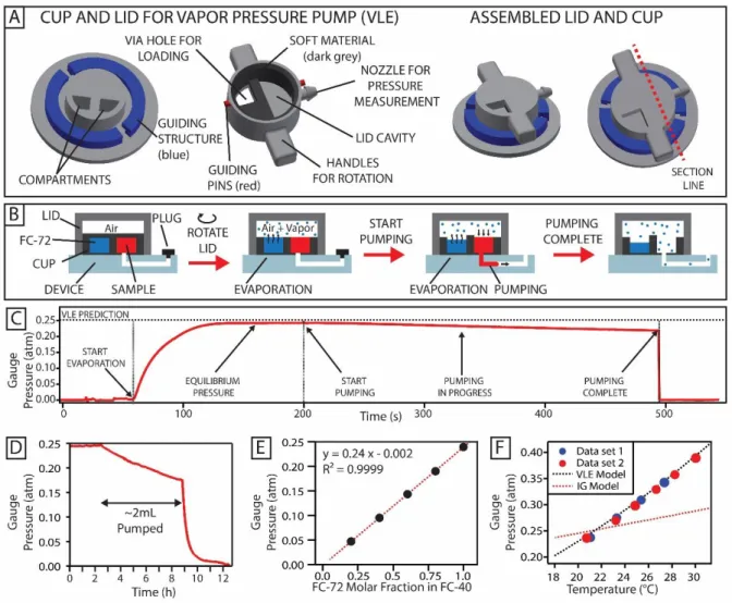
2.7 Generation of pressure using vapor liquid equilibrium (VLE) ... 24

S2.1 Schematic representation of the parameters used for the calculation of the positive pressure ... 35

S2.2 Schematic representation of the parameters used for the calculation of the negative pressure ... 36

TS2.1 Pressure measurements reported in Figure 1C ... 38

S2.3 Schematic of the experimental setup used for flow rate measurement ... 39

TS2.2 Properties of the liquids used in the flow rate experiments ... 40

TS2.3 Mean pumping times and mean experimental flow rate of nine sample types ... 41

TS2.4 Calculated flow rates for the five lids used in the laminar flow experiments ... 44

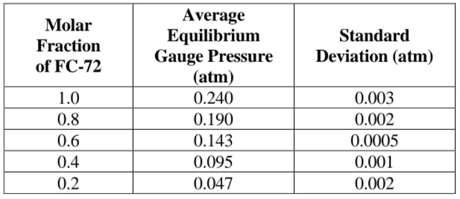
TS2.5 Experimental values for equilibrium pressures obtained with mixtures of FC-72 and FC-40 ... 46

TS2.6 Experimental gauge pressures at different temperatures ... 46

TS2.7 Predicted gauge pressures at different temperatures for FC-72 ... 47

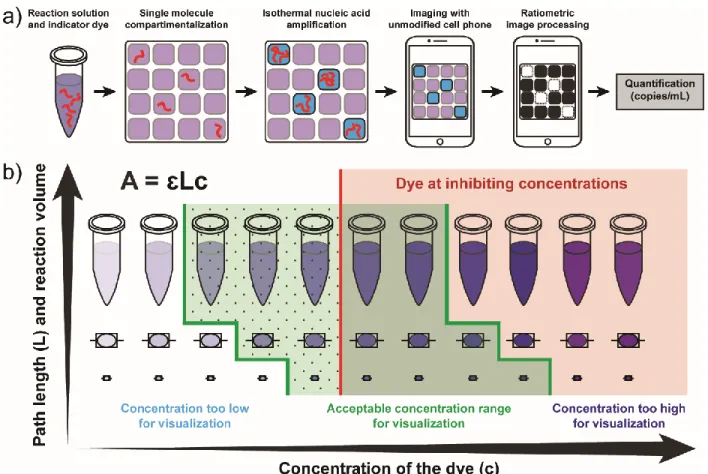
3.1 A visual readout approach for digital single-molecule isothermal amplification for use with an unmodified cell phone camera ... 52 3.2 Predicted values and experimental validation of the first step of the ratiometric approach . 55

(14)

3.3 Validation of the robustness of the G/R ratiometric approach to different hardware (cell

phone cameras) and lighting conditions ... 60

3.4 Readout from single-molecule digital LAMP reactions performed with λDNA on a multivolume rotational SlipChip device ... 62

3.5 Robustness of digital visual readout at different well volumes ... 64

3.6 Experimental validation of two-step SlipChip devices for single molecule counting with an unmodified cell phone camera ... 66

S3.1 DNA gel electrophoresis for RT-LAMP product ... 83

S3.2 Each step of the G/R process algorithm ... 84

S3.3 Original and G/R-processed images acquired with unmodified cell phone cameras ... 85

S3.4 Schematic of the top (left) and bottom (right) plates of the multivolume rotational SlipChip device used in the one-step digital LAMP experiments before being assembled ... 86

S3.5 Schematic of the multivolume rotational SlipChip device used for one-step digital LAMP experiments after being assembled ... 87

S3.6 Positive counts obtained from single-molecule digital LAMP reactions performed with lambda DNA on a one-step SlipChip device imaged by a house-built real-time fluorescence microscope, a Leica MZ Fl III stereoscope, and an unmodified cell phone camera (Apple iPhone 4S) under fluorescent light ... 88

S3.7 Five multivolume experiments were performed, and the concentration of each volume was calculated ... 89

S3.8 Performance of bulk LAMP reactions at increasing concentrations of the amplification indicator dye eriochrome black T (EBT) ... 89

S3.9 Schematic of the two-step SlipChip device before assembly ... 90

S3.10 Schematic of the two-step SlipChip device after assembly and its operation ... 91

TS3.1 Sequence of primers used in RT-LAMP experiments for detection of hepatitis C RNA .... 92

TS3.2 Sequence of primers used in LAMP experiments for detection of phage lambda DNA ... 92

TS3.3 Multivolume device designs for viral load quantification ... 93

S3.11 Measured spectral transmittance (%) in the range of visible light (400–700 nm) for positive (solid blue line) and negative (solid purple line) RT-LAMP reaction solutions ... 94

(15)

xv S3.12 Comparison of the spectral absorbance (Absorbance Units) of untreated indicator dye stock solutions (dashed orange lines) and solutions treated with Chelex® 100 resin ... 95 S3.13 Storage stability of amplification indicator dyes by drying the stock solutions in the presence of stabilizer trehalose ... 96 4.1 Diagram of the multistep SlipChip device illustrating the drop-in approach using back-and-

forth slipping in which the interfacial energy between two immiscible phases drives fluid transfer ... 102 4.2 Top-down view of two-row section of the multistep SlipChip device ... 106 4.3 A subset of the multistep SlipChip device (wells 10–20) showing overlaid fluorescence and bright-field images after each of seven drop-in and merging events ... 109 4.4 Reproducibility and spatial distribution of volume metering by carrier wells in the multistep SlipChip ... 111 4.5 Three-dimensional rendering of a two-well row section of the multistep SlipChip and a schematic illustrating the fragment barcoding process ... 113 4.6 An overview of device-performance metrics ... 115 S4.1 Photo of the multistep SlipChip ... 128 S4.2 Top-down view shows the two-row section of the multistep device performing evacuation of the loaded mixing wells ... 129 S4.3 A three-dimensional reconstruction of a droplet inside a 3-nL well from confocal Z-stack for volume calculation in Imaris ... 130 S4.4 Spatial distribution of barcoded reads within the device for repaired total human RNA experiment ... 131

(16)

CHAPTER 1 Introduction

Microfluidics, the study of fluids confined by sub-millimeter geometric features, has proved itself a useful set of tools for applications that are difficult to investigate with more traditional, macroscopic methods. Shrinking the experiments down produces multiple advantages, such as lower reagent volumes, shorter reaction times, and the potential for high-level multiplexing, to name a few.^1,2 With dimensions and volumes that approach those of the fundamental biological units themselves (e.g.

cells and macromolecules), microfluidics stands to benefit fields such as molecular diagnostics and single-cell omics (e.g. genomics, transcriptomics, and proteomics with single-cell resolution) in particular.

Since its inception, the field of microfluidics has amassed a wealth of capabilities and devices dealing with pressing challenges of biology, chemistry, and medicine. However, the fact that operation of many of these devices requires substantial additional equipment like pumps, power supplies, and signal readout instruments, has been commonly overlooked. Not surprisingly, the large size of these external appliances relative to microfluidic components themselves frequently undermines many of the practical benefits of assay miniaturization and claims to portability.³ The goal of the first two chapters of my thesis work has been to address these obstacles and to improve the stand-alone usability of microfluidic devices, in an effort of making them more portable and more friendly to resource-limited settings.

Chapter II addresses the challenge of pumping in microfluidic devices. Since many microfluidic workflows require stable pressure gradients and sample flows, not to mention sample loading before an assay can even begin, pumping method development has been an active area of lab-on-a-chip research.⁴ While good enough to demonstrate a proof-of-concept microfluidic device operation in lab, typical lab bench pumps are bulky, expensive, and power grid dependent. A portable version of a pump would be able to liberate microfluidic technology out of the labs where it is being developed into the labs of users (such as biologists and clinicians) and into a range of other applications in

(17)

2 resource-limited settings. In this previously published work on which I am a co-first author, we first theorize and then use multimaterial 3D printing to create and validate such pumping mechanisms.

We show that these pumps provide precise and predictable control of flow over a wide range of flow rates, independent of the sample’s volume, surface energy, and density. Also, unlike their classical counterparts, these pumps don’t have any moving parts—an important feature for applications requiring stable flows (e.g. droplet generation by flow focusing).⁵ We further demonstrate the utility of these 3D printed, attachable pumps with a variety of microfluidic devices, requiring both positive and negative relative pressures. We also show this technology’s sufficient robustness to operator error by asking an untrained 6-year-old user to load a device.

At the other end of a microfluidic assay workflow is the result readout. Making this part robust to the environment and the user’s level of training, while not requiring specialized equipment, is a significant challenge to democratization of lab-on-a-chip technology.⁶ Chapter III of this thesis presents previously published work (on which I am a contributing author) in which we demonstrate a quantitative, ultrasensitive microfluidic nucleic acid amplification test that permits the counting of single DNA and RNA molecules using an unmodified camera phone. This is accomplished by combining colorimetric indicator dye and a digital isothermal amplification strategy inside a microfluidic device, together with an image processing algorithm that converts the endpoint change in color into a ratiometric readout. The conversion of the colorimetric signal to its ratiometric alternative is central to the robustness of the method, since it normalizes for ambient lighting conditions. We also demonstrate that this is a hardware-agnostic approach by testing several smartphone cameras and imaging devices.

In addition to all the benefits of miniaturization mentioned above, microfluidic technology also holds the potential for integrating entire laboratory procedures on a single chip (hence the term lab-on-a- chip).⁷ In Chapter IV, I switch gears from the previous chapters and explore this angle. In this previously published work on which I am the first author, I present a versatile, SlipChip-based microfluidic platform as an approach for performing multistep biochemical reactions in a multiplexed format on a nanoliter scale. With its straightforward chip-to-world interfacing (requiring only pipette and manual operation), this technology provides an accessible approach that addresses

(18)

a previously unfilled niche in the reaction miniaturization field.³ We demonstrate the device’s functionality by performing a complex multistep biochemical scheme—barcode ligation of RNA transcripts for downstream multiplexed sequencing. Our comparative analysis shows that the multistep device’s performance is competitive with the current state of transcriptomic technologies.

This simple-to-use lab-on-a-chip technology for sequentially merging droplets in parallel will enable numerous applications, and will be particularly beneficial for protocols and biological assays such as biomarker detection, nucleic acid quantification, and time-sensitive reactions.

References

1. A. Folch, Introduction to bioMEMS, CRC Press, 2016.

2. D. J. Beebe, G. A. Mensing, and G. M. Walker, "Physics and Applications of

Microfluidics in Biology," Annual Review of Biomedical Engineering, 2002, 4, 261-286.

3. M. I. Mohammed, S. Haswell, and I. Gibson, "Lab-on-a-chip or Chip-in-a-lab:

Challenges of Commercialization Lost in Translation," Procedia Technology, 2015, 20, 54-59.

4. Y.-N. Wang and L.-M. Fu, "Micropumps and biomedical applications – A review,"

Microelectronic Engineering, 2018, 195, 121-138.

5. V. Gnyawali, M. Saremi, M. C. Kolios, and S. S. H. Tsai, "Stable microfluidic flow focusing using hydrostatics," Biomicrofluidics, 2017, 11, 034104.

6. E. Fu, "Enabling robust quantitative readout in an equipment-free model of device development," Analyst, 2014, 139, 4750-4757.

7. M. Boyd-Moss, S. Baratchi, M. Di Venere, and K. Khoshmanesh, "Self-contained microfluidic systems: a review," Lab on a Chip, 2016, 16, 3177-3192.

(19)

4

CHAPTER 2 The pumping lid: Investigating multi-material 3D printing for equipment-free, programmable generation of positive and negative pressures for microfluidic

applications

Abstract

Equipment-free pumping is a challenging problem and an active area of research in microfluidics, with applications for both laboratory and limited-resource settings. This paper describes the pumping lid method, a strategy to achieve equipment-free pumping by controlled generation of pressure.

Pressure was generated using portable, lightweight, and disposable parts that can be integrated with existing microfluidic devices to simplify workflow and eliminate the need for pumping equipment.

The development of this method was enabled by multi-material 3D printing, which allows fast prototyping, including composite parts that combine materials with different mechanical properties (e.g. both rigid and elastic materials in the same part). The first type of pumping lids we describe was used to produce predictable positive or negative pressures via controlled compression or expansion of gases. A model was developed to describe the pressures and flow rates generated with this approach and it was validated experimentally. Pressures were pre-programmed by the geometry of the parts and could be tuned further even while the experiment was in progress. Using multiple lids or a composite lid with different inlets enabled several solutions to be pumped independently in a single device. The second type of pumping lids, which relied on vapor-liquid equilibrium to generate pressure, was designed, modeled, and experimentally characterized. The pumping lid method was validated by controlling flow in different types of microfluidic applications, including the production of droplets, control of laminar flow profiles, and loading of SlipChip devices. We believe that applying the pumping lid methodology to existing microfluidic devices will enhance their use as portable diagnostic tools in limited resource settings as well as accelerate adoption of microfluidics in laboratories.

(20)

Introduction

This paper describes an equipment-free method for generating positive and negative pressures in a microfluidic device using a pumping lid. Most of the microfluidic devices developed in the past two decades rely on external equipment for operation, including the use of pumps, gas cylinders or other external controllers^1-5 for precise pumping and loading. Achieving the same degree of flow control without expensive or bulky equipment is necessary for making microfluidic devices more accessible. Currently, equipment-free pumping is both a challenging problem and an active area of research, with several proposed approaches.^6-15 For applications in which the total sample volume is less than the internal volume of the device, the sample’s surface energy is known and stable flow rate isn’t required, capillary-based pumping (wicking) can be used.^6-10 This has been done by flowing samples through microchannels^9,10 or using fibrous materials, such as paper.^6-8 For cases when the device can be pre-loaded with a solution, and the solution’s surface energy is known, the flow of the solution can be driven by the difference in capillary pressure between droplets of different sizes of this solution placed at the inlet and outlet of the device. For this method the pressure difference can be restored constantly by the addition of solution to the smaller droplet.^11,12 When only small sample volumes are used (a few microliters or less) and the application does not require flow rates greater than a few nanoliters per second, pre-degassed microfluidic devices can be used to generate flow.^13,14 Finally, when the density and volume of the sample are known, and the device can be stabilized in a precisely horizontal position, gravity can generate predictable pressure drops and drive the flow in a microfluidic device. In this approach, the difference in height of fluid in separate reservoirs generates the desired pressure drop.¹⁵ These methods have wide-ranging applications, but none can provide precise and predictable control of pumping in the absence of external equipment, independent of the sample’s volume, surface energy and density, while still achieving a wide range of flow rates.

Here we describe the theory, characterize the method, and validate the design of a range of equipment-free pumping lids for controlled-pressure generation in microfluidic applications. This pressure generation approach is based on controlled gas expansion or compression, so it does not depend on the nature of the liquid being pumped, the geometry of the channels, or the device’s

(21)

6 orientation. It can also be coupled with evaporation of a volatile liquid to generate pressure.

Development and characterization of this method was enabled by multi-material 3D printing which allows fast prototyping of composite parts that have sections with different mechanical properties.

In addition, the pumping lid approach has the following beneficial features that have not been combined previously in a single method:

a) The same setup can pump liquids of different density and/or surface energy with no difference in the resulting flow rate.

b) The pressure source is integrated with the device, so the method does not require the use of external connectors or tubing.

c) A simple model can be used to predict the pressure/flow rate generated by a specific lid/cup combination.

d) Pumping lids are interchangeable, so the same microfluidic device can be used with different lids to generate different flow rates. Pressures can be tuned by choosing the pumping lid with the appropriate dimensions and/or by modifying the lid’s geometry.

e) The user can alter the pressure by simply changing the position of the pumping lid, without interrupting the experiment.

f) Flow rates can be tuned precisely, with values ranging from a few nanoliters to more than a microliter per second, and remain consistent for long periods (hours in some cases).

g) The sample volume pumped can be larger than the internal volume of the device, making the method appropriate for handling samples that range from a few microliters to milliliters.

h) Both positive and negative pressures can be produced in predictable ways and used to generate and control flow.

i) While pumping is in progress, the lid keeps the sample isolated from the external environment, preventing contamination and evaporation.

j) The combined weight of all parts is less than 50 g, making it portable.

k) The device can be made of low-cost, disposable/recyclable polymeric materials, making it adaptable to resource-limited settings.

(22)

Results and discussion

Principle of pumping lid operation

The pumping lid method described in this paper is based on controlled compression or expansion of gas (Figure 2.1). To generate positive pressure, the user places the sample at the device inlet and then places the pumping lid on the cup integrated into the microfluidic device (Figure 2.1A). When the user pushes the lid down to its final position, the air in the lid’s cavity is isolated and compressed, creating positive-gauge pressure. The lid’s position is held by friction, but to increase robustness, guiding and locking structures can be integrated into the design (Figure 2.1A-B). Conversely, to create negative pressure, a pumping lid is pre-placed on the cup (Figure 2.1B) and the user pulls up on the pumping lid, expanding the air in the cavity. The degree of expansion is controlled by guiding structures.

(23)

8

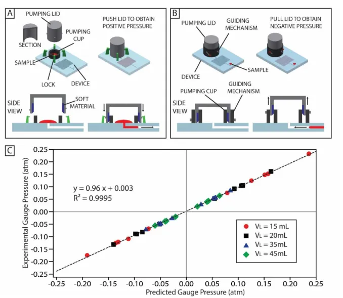
Figure 2.1 Principle of pumping lid operation. (A) Schematic of the method to generate positive pressure. A device is equipped with a cup (black) and locks (green). A sample (red) is placed in the cup before pumping. The pumping lid (grey) contains a cavity as shown in the side view. Part of the pumping lid is composed of a soft, deformable material (blue). Placing the lid on the cup compresses the air in the cavity and generates the pressure used to pump the sample in the device. The locks hold the lid in place to maintain the pressure over time. (B) Schematic of the method to generate negative pressure. The pumping lid (grey) is placed on the inner cup (black, visible only in the side view) before the experiment, and is equipped with guiding pins (red). These pins slide on a guiding structure (black) to guide the movement of the lid. When the user pulls the lid, the air in the cavity expands, creating a negative gauge pressure that pumps the sample into the device. (C) Pressures obtained from 40 experimental cup-lid combinations (N=3) plotted against the pressure values

(24)

obtained from the model (Eq. 2.2 and Eq. 2.6). The colors denote lids of different cavity volumes.

The dashed black line indicates the linear fit of the data and its parameters are reported in the graph.

Theoretical model for prediction of the pressure generated with the pumping lid

First, we analyze the initial pressure generated by the pumping lid and cup, prior to pumping. We use the Boyle law for isothermal gas compression: 𝑃₀𝑉₀ = 𝑃₁𝑉₁; assumptions of ideal gas behavior are appropriate in this case because the pressures are low (~ 1 atm) and the temperatures are sufficiently high (~ 300K).

Positive pressures

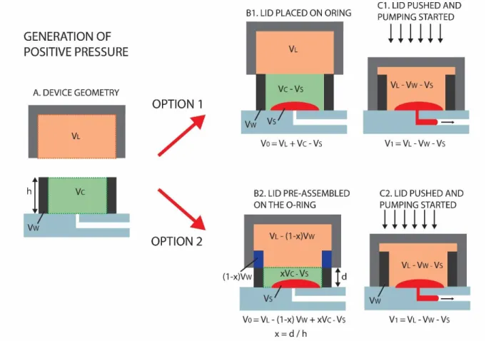
The positive pumping pressure depends on four main parameters: the volume of the cavity in the pumping lid (𝑉_𝐿), the volume of the cup walls (𝑉_𝑊), the volume of the empty space inside the cup (𝑉_𝐶), and the volume of sample loaded in the cup (𝑉_𝑆). When the lid is placed on the cup and first creates the seal, the volume of air enclosed is defined as 𝑉₀ = 𝑉_𝐿+ 𝑉_𝐶− 𝑉_𝑆, and the initial pressure is 𝑃₀ ~1 atm (Figure S2.1, Option 1). After the user pushes down the lid, the air is compressed and the final volume is given by 𝑉₁ = 𝑉_𝐿− 𝑉_𝑊− 𝑉_𝑆. Applying Boyle’s law, the pressure at this point is calculated as follows:

𝑃₁ =^𝑃^𝑂^(𝑉^𝐿^{+ 𝑉}^𝐶^{− 𝑉}^𝑆⁾

(𝑉_𝐿− 𝑉_𝑆− 𝑉_𝑊) = 𝑃_𝑂 + ^𝑃^𝑂^(𝑉^𝑊^+𝑉^𝐶⁾

(𝑉_𝐿 − 𝑉_𝑆− 𝑉_𝑊) (Eq. 2.1)

A more generalized formula can be used for the case when the lid is already pre-placed on the cup, at a distance 𝑑 from the final position (Figure S2.1, Option 2). The pressure is generated when the user pushes the lid to the final position. In this case, the pressure depends on the four volumes described above (𝑉_𝐿, 𝑉_𝐶 and 𝑉_𝑆, 𝑉_𝑊) and on the ratio 𝑥, between 𝑑 and the total height of the cup (ℎ), defined as 𝑥 = 𝑑/ℎ. The initial volume in this case is given by 𝑉₀ = 𝑉_𝐿 – (1 − 𝑥) 𝑉_𝑊+ 𝑥 𝑉_𝐶 – 𝑉_𝑆 and the initial pressure is again, the atmospheric pressure, 𝑃₀ ~ 1 atm. After the lid has been pushed down by a distance 𝑑, the final volume is given by 𝑉₁ = 𝑉_𝐿− 𝑉_𝑊− 𝑉_𝑆. The pressure at this point is calculated by using the same relation, 𝑃₀𝑉₀ = 𝑃₁𝑉₁, and is defined as:

(25)

10 𝑃₁ =^𝑃^𝑂^[𝑉^𝐿^{+x 𝑉}^𝐶^{−(1−x )𝑉}^𝑊^−𝑉^𝑆⁰^]

𝑉_𝐿− 𝑉_𝑊−𝑉_𝑆⁰ = 𝑃_𝑂+^𝑃^𝑂^x(𝑉^𝑊^+𝑉^𝐶⁾

𝑉_𝐿− 𝑉_𝑊−𝑉_𝑆⁰ (Eq. 2.2)

𝑉_𝑆⁰ defines the initial sample volume.

Second, we analyzed changes in pressure due to pumping. The pressure as a function of time is expressed as:

𝑃₁(𝑡) =^𝑃^𝑂^[𝑉^𝐿^{+x 𝑉}^𝐶^{−(1−x )𝑉}^𝑊^−𝑉^𝑆

0]

𝑉𝐿− 𝑉𝑊−𝑉𝑆(𝑡) (Eq. 2.3)

𝑉_𝑆(𝑡) defines the volume of sample present in the cup at time 𝑡. When the sample volume is substantially smaller than the difference between the cavity and pumping cup volumes, 𝑉_𝐿− 𝑉_𝑊, the change in the only time-dependent term, 𝑉_𝑆(𝑡), becomes negligible and the pressure can be considered constant, and Eq. 2.3 becomes identical to Eq. 2.2. This assumption was verified in all the experiments described in this paper, unless otherwise stated. Eq. 2.3 can be used to guide the design of pumping lids and cups, to predict the variation in pressure due to pumping and tune it, if needed.

When the sample volume is large enough to affect the pressure, the following set of equations can be used to describe the change in pressure. Given the hydraulic resistance (𝑅_𝐻) of the device, the time-resolved drop in positive pressure can be calculated as the sample is pumped out of the cup:

𝑃₁(𝑡) = ^𝑃⁰^(𝑉^𝐿^{−(1−𝑥)𝑉}^𝑊^+𝑥𝑉^𝐶^−𝑉^𝑆⁰⁾

√(𝑉_𝐿−𝑉_𝑊)²+2(^𝑃0𝑡

𝑅𝐻(𝑉_𝐿−(1−𝑥)𝑉_𝑊+𝑥𝑉_𝐶−𝑉_𝑆⁰)−𝑉_𝑆⁰(𝑉_𝐿−𝑉_𝑊−^𝑉𝑆 0 2))

(Eq. 2.4)

Eq. 2.4 is only valid for 𝑃₁ ≥ 𝑃₀ and while pumping is in progress. We assumed that the values of 𝑅_𝐻 remained constant in our experiments, because we pre-filled the channels with the solution being pumped. If the channel is not pre-filled, the initial variation of 𝑅_𝐻 during filling would need to be accounted for. To calculate the time required to pump the whole sample volume, the following equation is used:

(26)

𝑡^∗ =

(𝑉𝐿−𝑉𝑊−^𝑉𝑆 0 2)𝑉_𝑆⁰ 𝑃0

𝑅𝐻(𝑉_𝐿−(1−𝑥)𝑉_𝑊+𝑥𝑉_𝐶−𝑉_𝑆⁰) (Eq. 2.5)

Eq. 2.5 relies on the same assumptions as Eq. 2.4.

Negative pressures

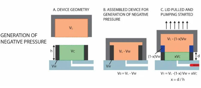
For generation of negative gauge pressures, the pumping lid is pre-placed onto the cup, and the user pulls it by a distance 𝑑. Assuming the cup is empty prior to pumping, the initial volume is given by 𝑉₀ = 𝑉_𝐿− 𝑉_𝑊. The initial pressure is the atmospheric pressure, 𝑃₀ ~1 atm. If the channel is not pre- filled with solution prior to pumping, the channel volume needs to be accounted for in 𝑉₀. After the lid has been pulled by a length 𝑑, the final volume of air is given by 𝑉₁ = 𝑉_𝐿+ 𝑥 𝑉_𝐶 – (1 − 𝑥) 𝑉_𝑊. Using previously defined parameters and the relation 𝑃₀𝑉₀ = 𝑃₁𝑉₁, the pressure at this point is defined as:

𝑃₁ = ^𝑃^𝑂^(𝑉^𝐿^{− 𝑉}^𝑊⁾

𝑉𝐿+x 𝑉𝐶−(1−x )𝑉𝑊 = 𝑃_𝑂− ^𝑃^𝑂^x(𝑉^𝑊^+𝑉^𝐶⁾

𝑉𝐿+x 𝑉𝐶−(1−x )𝑉𝑊 (Eq. 2.6)

Similarly to the case of the positive pressure, once pumping commences, the time dependence of 𝑃₁ is given by the expression:

𝑃₁(𝑡) = ^𝑃^𝑂^(𝑉^𝐿^{− 𝑉}^𝑊⁾

𝑉_𝐿+x 𝑉_𝐶−(1−x )𝑉_𝑊−𝑉_𝑆(𝑡) (Eq. 2.7)

𝑉_𝑆(𝑡) represents the volume of sample pumped into the cup at a given time 𝑡. When the sample volume is much smaller than 𝑉_𝐿+ x 𝑉_𝐶− (1 − x )𝑉_𝑊, the only time dependent term in Eq. 2.7, 𝑉_𝑆(𝑡), becomes negligible and the pressure can be considered constant. Whenever this assumption cannot be made, one can calculate the time-resolved drop in pressure as the sample is pumped into the cup, given the hydraulic resistance (𝑅_𝐻) of the device:

𝑃₁(𝑡) = ^𝑃⁰^(𝑉^𝐿^−𝑉^𝑊⁾

√(𝑉𝐿−(1−𝑥)𝑉𝑊+𝑥𝑉𝐶)²−2^𝑃0𝑡

𝑅𝐻(𝑉𝐿−𝑉𝑊) (Eq. 2.8)

(27)

12 Eq. 2.8 is only valid for 𝑃₁ ≤ 𝑃₀ and while pumping is in progress. To calculate the time required to pump a given sample volume one should use the following equation:

𝑡^∗ =

(𝑉𝐿+𝑥𝑉𝐶−(1−𝑥)𝑉𝑊−^𝑉𝑆 𝑓 2)𝑉_𝑆^𝑓 (𝑉𝐿−𝑉𝑊) ∙^𝑅^𝐻

𝑃0 (Eq. 2.9)

𝑉_𝑆^𝑓 represents the total sample volume to be pumped into the cup.

Generation of predictable positive and negative pressures

We experimentally tested (Figure 2.1C) predictions of the model for generating both positive (Figure 2.1A) and negative (Figure 2.1B) gauge pressures. We report (Figure 2.1C) the pressures obtained from 40 combinations of cups and pumping lids, plotted against the pressure value predicted by Eq.

2.2 and Eq. 2.6. Cups were 3D-printed directly on a rigid support and not connected to a device. We used a 5 psi differential pressure sensor (PXCPC-005DV, Omega Engineering), which was connected to a power supply (Portrans FS-02512-1M, 12V, 2.1 Amp power supply, Jameco Electronics) and to a data acquisition board (OMB-DAQ-2408, Omega Engineering). A custom program was written in LabVIEW (National Instruments) to convert the signal collected by the sensor to gauge pressure. The sampling frequency was 2 Hz. Each condition varied in at least one model parameter (𝑉_𝐿: 14.7 mL − 44.8 mL; 𝑉_𝐶: 0 − 2.7 mL; 𝑉_𝑊: 0.8 µL − 3.6 µL; 𝑥: 0.25 − 0.75).

The pumping lids used for these experiments included a nozzle that could be connected to the positive side of the pressure sensor using a short piece of Tygon tubing (1 cm long). Lid volumes were calculated using CAD software, accounting for the extra volume introduced by the nozzle, tubing, and the sensor. The other side of the sensor was exposed to the external environment, so all data collected were in terms of gauge pressure. The results were a close match to the predicted outcome, with an R² value of 0.9995 and a slope of 0.96. The pressures produced in this experiment spanned more than an order of magnitude (Table TS2.1). Furthermore, the model predicts that even higher pressure could be obtained by decreasing the volume of the empty parts (𝑉_𝐿, 𝑉_𝐶) and/or by increasing the other volumes (𝑉_𝑊 and 𝑉_𝑆).

(28)

Design guidelines for the pumping lid and cup

We found three guidelines to be helpful in designing pumping lids and cups: (1) the model can be used to either predict the pressure generated by a particular lid/cup combination, or to determine the lid and cup dimensions needed to achieve a particular pressure. All parameters can be tuned and the resulting pressure for each combination can be predicted using the equations described in the previous section. (2) To ensure effective sealing between the pumping lid and the cup, at least one of the two parts (lid or cup) should contain a deformable (soft) portion. The design requires a small overlap between the parts, so the soft portion is forced to deform when the lid is placed on the cup, thus creating a hermetic seal. Typical overlaps were in the order of 100 µm to 200 µm, which corresponds to ~ 1-2% of the cup diameter. We used multi-material 3D printing provided by Objet 260 system (Stratasys, Eden Prairie, MN, USA), which can produce parts composed of two different materials, and mixtures of these two materials. (3) Compression deforms the soft portion of the lid, and the material tends to be squeezed laterally. We observed that if this deformed material goes between the pumping lid and the base of the cup, the lid cannot be pushed to its final position and the obtained pressure will be lower than the one predicted by the model. This effect can be minimized by ensuring that the thickness of the soft layer is significantly larger than the overlap between the lid and cup, typically in the order of 1-1.5 mm. Another solution is to use soft layers with a tapered profile (Figure 2.1A).

Controlled pressure variation during an experiment

Next, we wished to test whether it would be possible to switch the pressure applied by the pumping lid without interrupting the flow or exposing the sample to the environment (to minimize contamination or evaporation). This capability is desired when several flow rates need to be tested in one continuous experiment. Pressure is changed by compressing or expanding air in the cavity.

Therefore, here we investigated whether the level of compression or expansion, and therefore the pressure, can be controlled precisely by using the guiding structures (Figure 2.2). For example, for both positive- and negative-gauge pressures, we designed lids that can be placed in three positions, labeled (a), (b), and (c). Each position provides a defined, specific pressure, and the user can switch between the positions by rotating the lid on its axis (Figures 2.2D, 2.2H). The lids for these

(29)

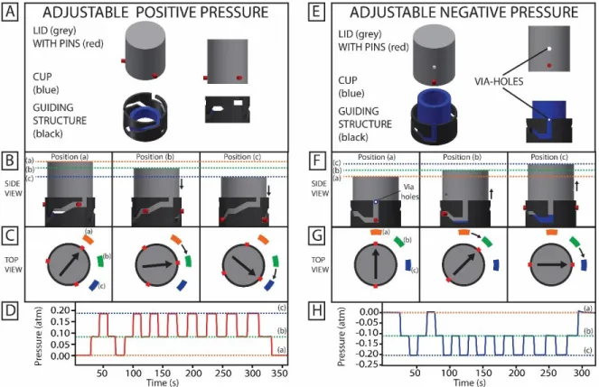
14 experiments were 3D-printed with a nozzle for the pressure sensor and pressure data was collected with the same setup as described in previous sections. For both positive- and negative-pressure devices, the starting position, (a), corresponds to zero gauge pressure (Figure 2.2). This adjustable design thus enables customized, “pre-programmed” pressure control during an experiment (e.g. to initiate or stop flow, and to change the flow rate) and allows the fully assembled device to be stored without applying pressure before use. While the devices demonstrated here are able to produce three specific pressures, more lid positions can be designed to enable finer tuning.

Figure 2.2 Strategies for producing multiple pressure values in a single device using a cup and pumping lid. (A-D) Positive pressures produced by turning a pumping lid (grey) using a cup (blue) fit with a guiding structure (black) (A). Turning the lid within the guiding structure yields three potential lid positions, which are shown in side (B) and top (C) views, each of which produces a different pressure. In Position (a), the lid is not in contact with the cup, so no pressure is produced.

In Position (b), the lid is lowered and positive pressure is produced. In Position (c), the lid is lowered further, and the pressure increases. The horizontal dashed lines show the level of the lid in the three

(30)

positions. Panel D shows an experimental pressure profile obtained by turning the lid between the three positions. (E-H) Negative pressures produced by turning a pumping lid (grey), using a cup (blue) fit with a guiding structure (black) (E). Turning the guiding structure yields three potential lid positions, which are shown in side (F) and top (G) views, each of which produce a different pressure.

The pumping lid and the cup have via-holes that align only in Position (a), so there is no gauge pressure in this configuration. In Position (b), the lid is raised and negative pressure is produced. In Position (c), the lid is raised further, and the pressure decreases. The horizontal dashed lines show the level of the lid in the three positions. Panel H shows an experimental pressure profile obtained by turning the lid between the three positions.

Generation of flow using the pumping lid approach

Next, we tested the prediction that for a given channel geometry, the pumping lid method would provide consistent flow rate that depends on viscosity, but not on surface energy or density of the fluid being pumped. We used Eq. 2.1 to predict the pressure applied by the pumping lid, and Eq.

2.10 to predict hydraulic resistance 𝑅_𝐻 that depends on the viscosity and the dimensions of the channel.¹⁶

𝑅_𝐻 = ^12µ𝐿

ℎ³𝑤(1−0.63(^ℎ

𝑤)) (Eq. 2.10)

𝐿 defines the channel length, ℎ the channel height, and 𝑤 the width of the channel. The volumetric flow rate can thus be predicted with Eq. 2.11:

𝑄 = ^𝑃

𝑅_𝐻=^𝑃ℎ

3𝑤(1−0.63(^ℎ 𝑤))

12µ𝐿 (Eq. 2.11)

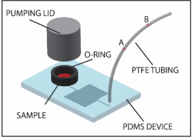
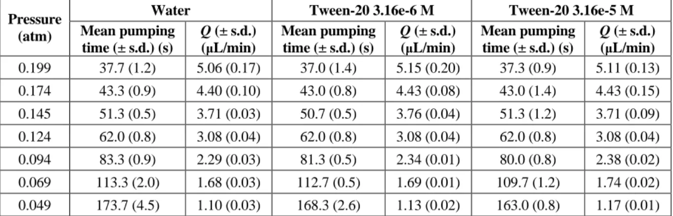
To test these predictions, we first characterized pumping of water through a microfluidic device using seven pumping lids, each providing a different pressure (Figure 2.3A). The device consisted of glass-bonded PDMS layer¹⁷, pumping cup, PTFE tubing, and the pumping lid (Figure S2.3). A

(31)

16 30.8 cm long, 58 µm high, 110 µm wide serpentine was molded into the PDMS layer, and was pre- filled with each solution prior to pumping experiment, as described in SI. The slope of the fitting curve is the inverse of the hydraulic resistance (𝑅_𝐻) for the experimental setup, as suggested by Eq.

2.11.

The experimental value for 𝑅_𝐻 obtained from the fit is 2.59*10¹⁴Pa s /m³, which matched the theoretical value calculated for the microfluidic channel geometry: 2.58*10¹⁴Pa s /m³.¹⁶ Thus, it was possible to predict the flow rate for a given pumping lid used with a given microfluidic device, and the design was robust enough to give reproducible results. The flow rates in this experiment were 1 – 5 µL/min, and this range was chosen to minimize the experimental errors when measuring flowing time. Higher flow rates could be produced by increasing the pressure generated by the pumping lid (as described in the previous sections), or by using a device with lower hydraulic resistance. For example, a device with a channel 150 µm tall x 150 µm wide x 20 mm long will have a hydraulic resistance almost 200 times less than the devices used for these experiments, so the flow rate generated with the same pumping lids would approach 1 mL/min.

(32)

Figure 2.3 Experimentally and quantitatively testing the model describing pumping with a pumping lid as a function of hydraulic resistance of the channel and properties of the fluid. (A) Flow rate of water in a microfluidic device using different pumping lids to generate different pressures. The dotted red line indicates the predicted flow rate based on the device geometry, while the dotted blue line shows the linear fit of the data; its parameters are reported on the graph (N=3;

error bars smaller than the size of the marker). (B) A plot of experimental flow rates, multiplied by the viscosity, for different aqueous solutions. Flow rates were inversely proportional to viscosity and independent of the surface energy or density of the solutions. Schematics of the setup used for these experiments are provided in the supplementary material. (Figure S2.3).

Generation of flow rate independent of density and surface energy

To verify that the flow rate in the pumping lid method is independent of solution density and surface energy, we pumped nine aqueous solutions of different properties (Table TS2.2) using seven different lids to measure the flow rate at different inlet pressures. Solutions of viscosity similar to water, but with different surface energies (30 – 72 mN/m) and different densities (1 – 1.9 g/mL), had flow rates comparable to those obtained for water. We experimentally measured viscosities of all nine solutions to confirm this result. Note that the viscosity-adjusted flow rate values (𝑄 ∙ 𝜇) were similar for all liquids (Figure 2.3B), which is explained in the next section.

Generation of flow for solutions of different viscosities

We then tested whether the pumping lid is appropriate to produce flow in solutions with viscosities higher than that of water. In our experiments, solutions had viscosities between 1 mPa*s and 4 mPa*s (Figure 2.3B). The flow rates for high viscosity solutions were lower than those obtained for pure water, because the value of the hydraulic resistance 𝑅_𝐻 described above is directly proportional to the viscosity of the liquid pumped (Eq. 2.10)¹⁶. Eq. 2.11 can be re-written as:

𝑄 ∙ µ = ^𝑃ℎ

3𝑤(1−0.63(_𝑤^ℎ))

12𝐿 (Eq. 2.12)

(33)

18 Eq. 2.12 predicts that, if the same lid-cup combination is used on the same device, the product of the flow rate and the viscosity of the solution will be constant.¹⁶ Our experimental results (Figure 2.3B) corroborated this prediction, since the µ ∙ 𝑄 values for all the solutions analyzed were comparable to those obtained for water (Figure 2.3B). This means that the pressure generated by a pumping lid depended solely on the lid-cup dimensions, and not on the nature of the solution to be pumped.

Use of multiple lids on the same device to achieve complex flow control over long timescales Next, we tested the idea that using separate cups and lids at different inlets makes it possible to simultaneously pump more than one solution and to independently control the pressure imposed at each inlet (Figure 2.4A). First, we used multiple lids to produce nanoliter droplets (Figure 2.4B).^18-

20 Immiscible fluids can be difficult to handle under pressure-driven flow because the applied pressure should be higher than capillary pressure but not so high to generate an excessive capillary number that would cause droplet deformation²¹. Also, when multiple inlets are controlled with different pressures, liquid could potentially flow from one cup to another. To avoid this, we designed devices with geometries that included a serpentine channel between the inlets and the junction used to produce the droplets. This serpentine channel had a fluidic resistance higher than that of the outlet channel, and ensured that liquids were not transferred from one cup to the other during experiments.

This approach was used to generate nanoliter droplets (plugs) of water in fluorinated oil, using flow focusing and T-junction geometries (Figure 2.4B), with volumes that ranged from 0.5 to 2.5 nL.

Parallel laminar flow profiles can also be produced (Figure 2.4C). We achieved stable flow patterns for more than 2.5 h, with a total pumped amount of 0.9 mL. The predicted decrease of flow rate in this system over a 2.5 h period was 45% of the original value (Eq. 2.4), which was consistent with our experimental observations (Figure 2.4C). Increased diffusion between the dyes was observed, due to the longer residence time in the channel. Because we used lids of the same size and loaded samples of the same volume and viscosity, over time we observed a decrease in the absolute value of the flow rates, but not a decrease in their ratios. We emphasize that if the volumes of the lids, cups, sample volumes and/or viscosities are different, the flow rates will drop at different rates (Eq.

2.4).

(34)

Figure 2.4 Use of the pumping lid approach to control pumping of each of several fluids with different properties in a microfluidic device. (A) Schematic of the pumping approach using multiple solutions in the same device. Each sample was pumped in the device with a different pumping lid, each lid producing a different pressure. (B) Left: Experimental photographs illustrating production of nanoliter plugs (red) in fluorinated oil (transparent), using a microfluidic device with flow focusing geometry. Right: Production of multicomponent aqueous droplets in fluorinated oil using a T-junction. The solutions (red, transparent and green) were pumped independently and used to produce nanoliter plugs. (C) Experimental photographs illustrating that the parallel laminar flow profile of three separate streams of aqueous solution (red, transparent and light blue) was stable even after 165 min (2.75 h). A total volume of 0.9 mL (300 µL of each solution) was pumped in this experiment.

Use of composite lids to produce different flow patterns in the same device

A “composite lid,” a pumping lid with multiple cavities, was designed to simultaneously seal multiple cups (Figure 2.5). The cavities in the composite lid can be isolated or connected to one another. For example, if inlets require identical pressures, their corresponding cavities can be linked (Figure 2.5C).

(35)

20

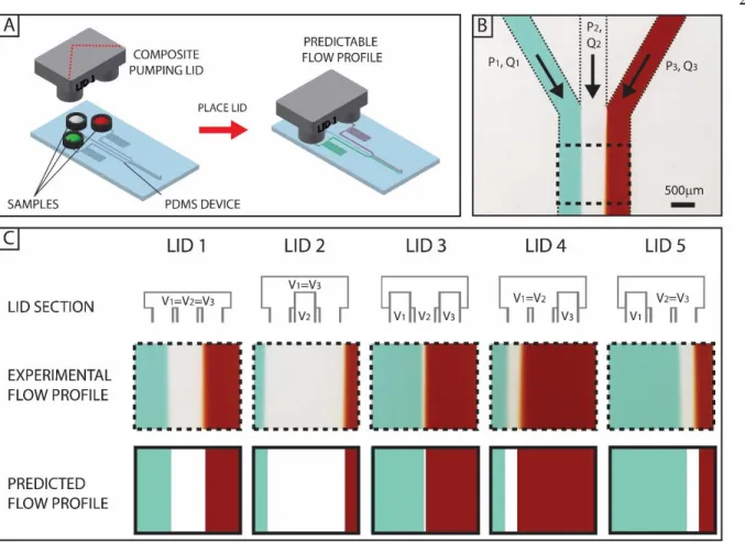
Figure 2.5 Production of different flow profiles in the same device using composite pumping lids. (A) Schematics of the setup used for the experiments. The microfluidic device has three cups, each dedicated to a different aqueous solution (from left to right: green, transparent, and red). A composite lid controls the pressure at each of the three inlets, thus controlling the flow rate of each solution. (B) Micrograph of the junction at which the three inlet branches combine into a single channel and the streams from the three inlets produce parallel laminar flow. (C) Different composite lids can be used to produce different flow profiles. The top row shows the cross-section of five different lids, cut along the red dashed line in panel A. The middle row shows the experimental flow profiles obtained with these five lids in the same microfluidic device. The sketches (bottom row) show the expected flow profiles based on the pressures produced by the lids and the device geometry.

For the channel used in these experiments, the width (1.5 mm) was more than 35 times bigger than the channel height (40 µm), so the effect of parabolic flow near the lateral walls was negligible.¹⁶

(36)

To test these devices quantitatively, we measured the width of each solution stream in the three- stream aqueous laminar flow, (the Reynolds number was always less than 1 in our experiments). The gauge pressures at the three inlets are defined as 𝑃₁, 𝑃₂, and 𝑃₃, while the pressure at the device outlet is zero. Fluidic resistances for the three inlet branches (before the junction) are defined as 𝑅, while the resistance of the main channel (formed by the junction of the three inlet branches) is defined as 𝑟. In the experiments described in this paper, the fluidic resistance 𝑅 of the inlet branches was intentionally set larger than the outlet resistance 𝑟, to increase the range of pressures that could be applied to the three inlets without generating back-flow in the branch with the lowest pressure. Under these conditions, theory predicts that 𝑄_𝑖 is proportional to 𝑃_𝑖 and can be approximated by Eq. 2.11.

Ignoring the effects of three-dimensional diffusion^22,23 and ignoring the effect of the parabolic flow profile for these wide channels, we predicted the flow profiles as described in the supplementary material, and found them to be in good agreement with experiments.

These lids were used to produce parallel laminar flow profiles in a microfluidic device (Figure 2.5B).

Each composite lid had a different geometry (Figure 2.5C) and generated a different set of pressures at the three device inlets. These pressures were used to predict the flow profile in the microfluidic device, as described in the supplementary material, and experimental results matched the flow profiles predicted by the flow rate model (Figure 2.5C). Based on the geometries of the device and the composite pumping lid, flow profiles can be controlled and predicted.

Use of pumping lids to load SlipChip devices by positive and negative pressures

Next, we showed that the pumping lid could be used to reliably and easily load SlipChip devices²⁴ using either positive or negative pressures. This is a good test because loading SlipChip devices requires control of the inlet pressure within a defined range,²⁵ and SlipChips are intended to be used in limited resource settings (LRS) by untrained users.^26-29 First, we tested the pumping lid on a SlipChip designed for a digital nucleic acid detection assay²⁶ (Figure 2.6A), pumping a total of 5 µL of solution with 0.03 atm pressure (Eq. 2.1). We asked a 6-year-old volunteer to use the pumping lid to operate the device. We found that pumping proceeded to completion despite the variation of

(37)

22 pressure applied to the pumping lid by the volunteer.^30,31 We expect the simplicity of the pumping lid to be valuable in both LRS and laboratory settings, e.g. for digital single-molecule measurements.³¹

In another experiment, we tested loading of a different SlipChip device by negative pressure. To further illustrate the applicability of the pumping lid method to complex tests, we used a SlipChip designed for multivolume digital nucleic acid amplification,^32,33 which presents challenges in filling due to variation of capillary pressure among wells of different sizes. Previously, this type of device was filled by positive pressure and dead end filling.²⁵ We modified the device for negative-pressure filling by adding a sealing ring filled with high-vacuum grease (sealing structure) around the active area containing the amplification wells (Figure 2.6B). We also added an outlet for oil to the device, over which the negative-pressure pumping lid was placed. The device was assembled such that the lubricating oil (5 cSt silicone oil) was filling the wells. For loading, sample (50 µL of 0.5 M FeSCN aqueous solution) was placed onto the inlet, and the pumping lid was pulled up to create negative pressure of 0.1 atm, remove excess oil and draw the sample into all of the wells of the device (Figure 2.6B). This experiment demonstrated that bubble-free filling can be accomplished using the pumping lid, and that complex devices (a combination of immiscible fluids and wells with different capillary pressures) can be handled.