This thesis could not have been written without the support of the many people who helped me during my research at the Kellogg Radiation Lab. Many thanks also go to Stefan Schmidt, from Ruhr-Universitiit Bochum, Germany, for creating the implanted 22Ne targets used in the second half of my final project.
List of Tables
- Supernovae and 22 Na Production
Recent computer simulations of explosive hydrodynamics and nucleosynthesis in Type II supernovae, performed by Woosley and Weaver [Woo95] and Thielemann, Nomoto and Hashimoto [Thi96], give the amounts of 22Na that would be produced in a supernova depending on the initial conditions of the star. Observational constraints on the amount of 22Na produced m supernovae can serve to verify these theoretical models.
There is a discussion of the differences between the theoretical models for the two groups in the Woosley and Weaver paper.). However, Woosley and Weaver [Woo80] note that because of the short half-life of 22Na, a calculation of the I transport in the expanding supernova remnant is required for a meaningful analysis of the yield of I rays from 22Na that might be expected. to observe given these ejected masses.
Chapter 2 Theoretical Overview
- Reaction Kinematics
- Cross Sections and Resonance Strengths
- Experimental Yields
- Reaction Rates
- Chapter 3 Experimental Overview
- Previous Work
- Scope of this Work
Writing Ptab in terms of Etat, the total energy of the particle in the laboratory frame, . The energy of the third particle in the laboratory frame is given by the usual Lorentz transformation.
Part II
Chapter 4 Pelletron Beams
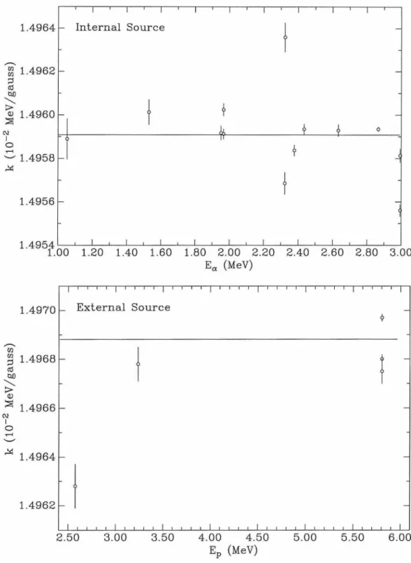
The beam energy, Ezab, is related to the analyzer magnet field z. From these measurements, k was found to be MeV/gauss, with the error calculated from both these measurements and the reproducibility of the resonance energies observed from the 22Ne(p, n)22Na measurements.
LJLJ
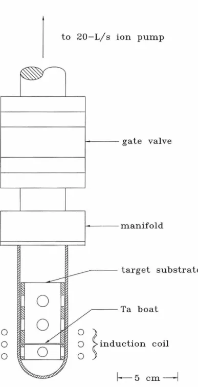
During bombing, the rear of the target was cooled with flowing liquid Freon (1,1,2-trichloro 1,2,2-trifluoroethane). The beam-induced fluorescence in the quartz showed the image of the collimator on the target.
5. 2 Target Installation
Chapter 6 Neutron Detection
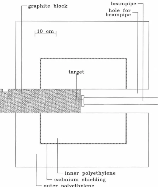
- Description of Polycube
- Background
- Deadtime
- Monte Carlo Simulations with MCNP
- Overview of MCNP
- Installation of MCNP
- Input Files and Detector Geometry
- Validation of MCNP Efficiencies
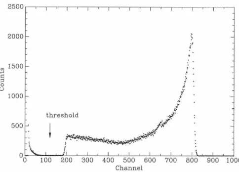
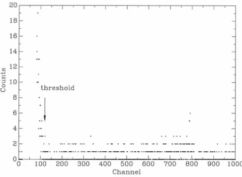
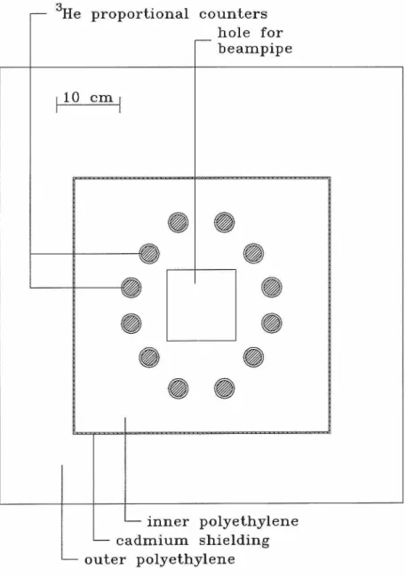
The peak corresponds to the deposition of the full value of Q (764 ke V) from the back proton and triton from the 3He(n, p)3H reaction. Therefore, the threshold is set at the center of the bottom between the noise peak and the neutron signal, as shown in Figures 6.3 and 6.4. The 3He pressure in the proportional counters was 4 atm according to the manufacturer's specifications.
The 3He listed above is the 3He in the active volumes of the meters, and the stainless steel is the housing steel of the proportional meter. The source capsule geometry was also included in the simulation, and the resulting MCNP performance is in excellent agreement with the experimental value. The weak source was then placed at the center of the polycube in the usual counting geometry and the efficiency of the cube was found to be 0.155(6).
This spectrum is calculated from the distribution of a particles from 241 Am and the cross section i.
- Results of the MCNP Simulations
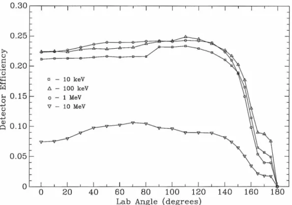
Note that the shape of the intercept curve is much more accurately reproduced by the MCNP efficiency than by the constant efficiency. For the readability of the graph, my data points are not shown, only straight lines connecting the points. As can be seen from the plot, MCNP mimics the shape of the curve quite well, with an absolute mean deviation of 1.6% from the Gibbons and Macklin sections and a maximum deviation of 5.0% for Ep 2: 1.887 MeV.
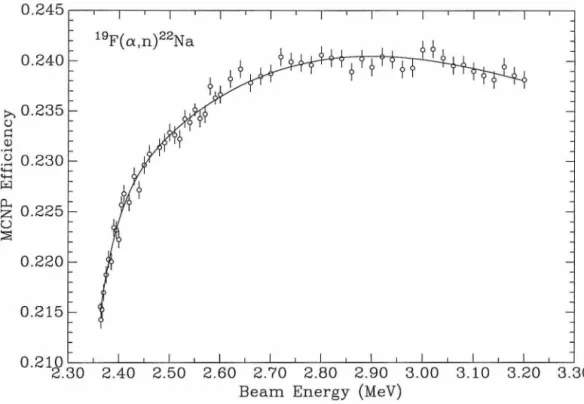
Since no angular distribution measurements are available for 19F(a, n)22Na, the normalization uncertainty of the MCNP efficiency is 4%. The upper plot in the figure shows the calculated yields for neutrons n0 and the corresponding fit to the data using an exponential and a polynomial. The total efficiency of neutrons above the threshold n1 was therefore chosen as the average efficiency of the available groups of neutrons.
The bottom plot shows all fits to the individual neutron groups as dashed lines, with the total neutron efficiency as a solid line.
![Figure 6.6: The 7 Li(p, n) 7 Be yield divided by the detector efficiency vs.beam energy, normalized to the Gibbons and Macklin [Gib59] cross sections](https://thumb-ap.123doks.com/thumbv2/123dok/10403001.0/54.857.127.741.292.718/figure-divided-detector-efficiency-normalized-gibbons-macklin-sections.webp)
Chapter 7 Gamma Ray Detection
- The BGO Detector
- The Ge Detector
The distance between the front of the casing surrounding the Ge was placed cm from the target. Since the two row beams of interest are so similar in energy (440 keV for the 22Ne(p, ry)23Na reaction and 444.0 keV for the . 152Eu source), no correction was made for this slight change in energy.
Chapter 8 Experimental Procedures
- Target Preparation
- Target Thickness Determination
- Target Contamination
- Yield Measurements
The slices were then rinsed in deionized water and mounted inside the target production apparatus. Bec82].* The normalization uncertainty of the results is estimated to be 7.0%, almost entirely due to the 6% in the BGO efficiency and the 3.6% error in the resonance strength. For the data analysis, target degradation was assumed to be linear with accumulated charge.
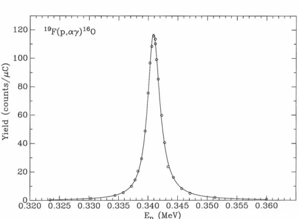
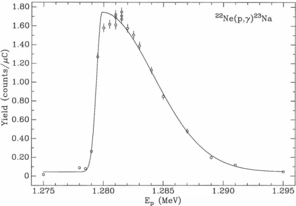
The solid curve is the fit to the data with an asymmetric Breit-Wigner function (two truncated Breit-Wigners joined at their peak), no background, and was used to determine the target thickness. The solid curve is the fit to the data of a Breit-Wigner function, and was used to determine the target thickness. The solid curve is the fit to the data of a Breit-Wigner function, and is used to determine the target thickness.
The amount of 180 in the target was found using the same method as for 13C: the 1.864-MeV resonance was used, with a (w'Y)r derived from the cross-section curve measured by Bair and Haas [Bai73].
Chapter 9 Data Analysis and Results
9 .1 Calculation of Cross Sections
Comparison with Existing Data
All resonances were fitted with a combination of Breit–Wigner (BW) or Gaussian functions with a linear background. Those peaks marked as asymmetric were fitted with two truncated Breit-Wigner or Gaussian functions concatenated at their peaks. a) average of three measurements from the same target. The laboratory energy and associated error are the values returned from the fit; there is a surcharge of 0.05%.
The true resonance energy will be less than the laboratory energy by approximately half the target thickness ke V at 2.36 Me V). The error quoted in Ex is the total error from my data, including statistical and systematic errors, but excluding the error in nuclear masses. The solid curve represents the target thickness yields calculated from my cross sections and the dotted lines represent the associated error bars.
However, there is a good correspondence in the energies for the resonances observed across the cross section and at 0°.
Thick Target Yields
According to the Balakrishnan cross-section [Bal78], the cross-section drops from 25 mb at the resonance at 3.3 MeV to less than 2 mb at 3.1 MeV, and extrapolation from higher cross-sections may not adequately reflect this drop-off.
Calculation of Reaction Rates
- Comparison with Hauser-Feshbach Calculations
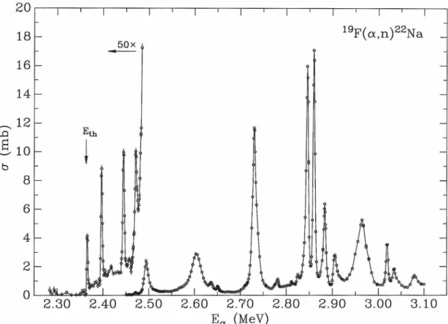
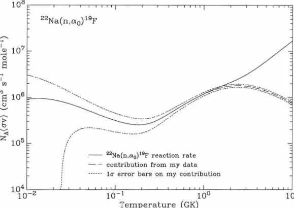
Na threshold is at 3.07 MeV, the above approach to extend the range of the cross section to my data gives the total 19F(a, n)22Na cross section and reaction rate. To determine the reaction rate for 19F( a, n0 )22Na alone, for the purposes of detailed balance, only ~ of the estimated cross section above 3.1 MeV is assumed to be due to n0 neutrons. As can be seen from the graph, the diameter within my range of energy accounts for 95% of the reaction rate below 1.4 GK and 50% below 3.2 GK.
The first term represents the contribution of a smoothly varying cross-section, while the next three terms represent resonances in the cross-section from my field of energies. The last term represents the contribution of the approach that increases the reach of the cross-section above my energies. The error for my contribution to the reaction rate includes all statistical and systematic errors in the cross-section.
In Figure 9.8, the reaction rate derived from my data is plotted against the semiempirical reaction rate calculated from Hauser-Feshbach models by Woosley et al.
Part IV
Chapter 10 Experimental Procedures
- Target Preparation
- Target Thickness Determination
- Yield Measurements
- Target Contamination
The target thickness was determined using two different methods: the detection of the /" rays from the 22Ne(p, 1)23Na reaction, and the detection of the neutrons from the 22Ne(a, n)25Mg reaction. This same resonance was measured in the same geometry for the thinner 22Ne target, so that its thickness could be determined from the thickness of the thicker 22Ne target Neutron yields of the thinner 22Ne target were measured for resonances at five energies whose width was comparable to the thickness of the thicker 22Ne target.
Since no structure is seen in the recovery of the Ta blank, this suggests that the contaminant is distributed throughout the support. The substrate yield also contains the contribution of neutrons created by the beam hitting the tantalum collimator. Background due to unknown contaminant(s) in the Ta substrate was then subtracted from the raw yield from the thicker 22Ne target.
The bottom graph shows the neutron yield of the same target after subtracting the yield of the contaminant from the Ta blank.
Chapter 11 Data Analysis and Results
- Calculation of Cross Sections
- Comparison with Existing Data
- Calculation of Reaction Rates
- Comparison with Experimental Rates
The laboratory energy and associated error are the values returned by the fit; there is an additional 0.1% uncertainty due to the energy calibration. The figure shows the cross sections above En = 0, while the inset plot shows the cross sections expanded around En = 0. The reaction rate NA ( Above the range of my data the cross section was expanded using the data measured by Takacs et al. [Tak96], but since the cross section below 5.4 MeV accounts for 100.% of the reaction rate at 10 GK. The first term represents the contribution of a slowly varying cross-section, while the next two terms represent resonances in the cross-section. Instead, I integrated the cross sections for 22Ne(p, n)22Na below the n1 threshold using Equations 2.27 and 11.2 to determine the contribution to the velocity of the cross sections within that range of energies, thus establishing a lower bound for the reaction speed. The fact that their velocity is much higher than my lower limit in the overlap region is consistent with their finding from their cross-sections that the velocity is dominated by the p1 channel. A remeasurement of the cross sections above the limit for this experiment, to improve the Balakrishnan data, would be useful to establish the reaction rate above 1.0 GK. For the 22Na(n, a0)19F cross section and velocity, it would be useful to measure the ratio of the n1 to n0 neutrons above the n1 neutron threshold at 3.07 MeV. Bibliography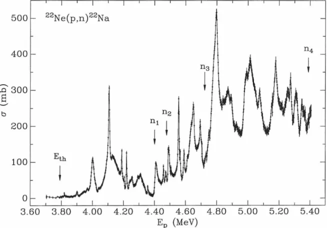
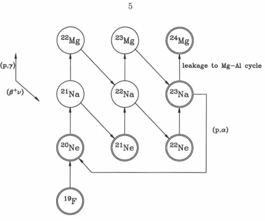
Chapter 12 The 19 F(a,n) 22 Na Reaction