Foraminiferal Densities and Pore Water Chemistry in the

(1)

Foraminiferal Densities and Pore Water Chemistry in the

Indian River, Florida

i — - w

M P •

m^*' '• «-

MARTIN A. BUZAS and

KENNETH P. SEVERIN

..jutmttr • v , * * - ^ * ^ ^ * * ^ ^ " * * ^ " ' " '

H ' I •Wr"*>

SMITHSONIAN CONTRIBUTIONS TO THE MARINE SCIENCES * NUMBER 36

(2)

Emphasis upon publication as a means of "diffusing knowledge" was expressed by the first Secretary of the Smithsonian. In his formal plan for the institution, Joseph Henry outlined a program that included the following statement: "It is proposed to publish a series of reports, giving an account of the new discoveries in science, and of the changes made from year to year in all branches of knowledge." This theme of basic research has been adhered to through the years by thousands of titles issued in series publications under the Smithsonian imprint, commencing with Smithsonian Contributions to Knowledge in 1848 and continuing with the following active series:

Smithsonian Contiibutions to Anthropotogy Smithsonian Contributions to Botany Smithsonian Contributions to tiie Earth Sciences Smithsonian Contributions to the Marine Sciences

Smithsonian Contributions to Paleobiology Smithsonian Contributions to Zoology

Smithsonian Folklife Studies Smithsonian Studies in Air and Space Smithsonian Studies in History and Technology

In these series, the Institution publishes small papers and full-scale monographs that report the research and collections of its various museums and bureaux or of professional colleagues in the world of science and scholarship. The publications are distributed by mailing lists to libraries, universities, and similar institutions throughout the world.

Papers or monographs submitted for series publication are received by the Smithsonian Institution Press, subject to its own review for format and style, only through departments of the various Smithsonian museums or bureaux, where the manuscripts are given substantive review.

Press requirements for manuscript and art preparation are outlined on the inside back cover.

Robert McC. Adams Secretary

Smithsonian Institution

(3)

S M I T H S O N I A N C O N T R I B U T I O N S TO THE M A R I N E S C I E N C E S • NUMBER 36

Foraminiferal Densities and Pore Water Chemistry in the

Indian River, Florida

Martin A. Buzas and Kenneth P. Severin

SMITHSONIAN INSTITUTION PRESS Washington, D.C.

1993

(4)

A B S T R A C T

Buzas, Martin A., and Kenneth P. Severin. Foraminiferal Densities and Pore Water Chemistry in the Indian River, Florida. Smithsonian Contributions to the Marine Sciences, number 36, 38 pages, 32 figures, 29 tables, 6 appendices, 1993.—Two stations were established about 10 m apart at a depth of about 1 m at Link Port, Florida. One consisted of quartz sand and the other of quartz sand with a dense stand of seagrass. At the surface of each station and at a depth of 10 cm at the grass site, four replicate samples consisting of 5 ml each were taken every fortnight from 27 March to 6 November 1978 (17 sampling times, 204 samples). The taxa Quinqueloculina, Elphidium, Ammonia, Bolivina, and Ammobaculites comprising 98% of the fauna were enumerated. In addition, pore water chemistry was measured for temperature, salinity, oxygen, pH, Eh, NH3, P04, Si, N02, and N 02 + N03.

General linear models were used to analyze the bare surface-grass surface, and grass surface-grass 10 cm data sets. Foraminiferal densities were evaluated for differences between sites, periodicity, sites x periodicity (interaction), and environmental variables.

Differences in overall density between the bare surface-grass surface sites were not significant for the three most abundant taxa (Quinqueloculina, Elphidium, and Ammonia). At the grass site the density for all taxa were significantly lower at 10 cm than at the surface (very few individuals were observed at 10 cm).

Hypotheses for periodicity and interaction were significant for all taxa in all comparisons except for Bolivina in the bare surface-grass surface analysis. At the bare surface, maximum densities occurred in spring while at the grass surface in summer. Although densities were low at 10 cm, no synchronization between the grass surface and 10 cm was evident.

The environmental variables were significant for all taxa in both comparisons. The environmental variables are, however, highly correlated. To alleviate this difficulty, a principal component analysis was performed on these variables. The first three components included all of the 10 variables. Subsequent multiple regression of foraminiferal densities and the principal components indicated that usually at least two components, accounting for most of the variables, were statistically significant. Thus, no simple relationship between pore water chemistry and density is apparent. The very large difference in density between the grass surface and 10 cm depth is much more strongly related to the pore water chemistry than the smaller differences with time at the surface sites.

OFFICIAL PUBLICATION DATE is handstamped in a limited number of initial copies and is recorded in the Institution's annual report, Smithsonian Year. SERIES COVER DESIGN: Seascape along the Atlantic Coast of eastern North America.

Library of Congress Cataloging-in-Publication Data Buzas, Martin A.

Foraminiferal densities and pore water chemistry in the Indian River, Florida / Martin A. Buzas and Kenneth P. Severin.

p. cm.—(Smithsonian contributions to the marine sciences ; no. 36) Includes bibliographical references (p. ).

1. Foraminifera—Florida—Indian River. 2. Protozoan populations—Florida—Indian River. 3. Population density—Florida—Indian River. 4. Pore water—Florida—Indian River. I. Severin, Kenneth P. II. Title.

III. Series.

QL368.F6B875 1993 593.1'2O4526323'097592-dc20 92-46076

® The paper used in this publication meets the minimum requirements of the American National Standard for Permanence of Paper for Printed Library Materials Z39.48—1984.

(5)

Variables 15 Quinqueloculina 15 Elphidium 16 Ammonia 16 Bolivina 21 Ammobaculites 22 Comparison of Analyses 23 Comparison with Other Studies 24 Appendix 1: Bare Surface 29 Appendix 2: Grass Surface 31 Appendix 3: Grass 10 cm 33 Appendix 4: Bare Surface 35 Appendix 5: Grass Surface 36 Appendix 6: Grass 10 cm 37

Literature Cited 38

in

(6)

(7)

Foraminiferal Densities and Pore Water Chemistry in the

Indian River, Florida

Martin A. Buzas and Kenneth P. Severin

Introduction

A basic variable for ecological studies is density, the number of individuals per volume or area. Densities of foraminiferal species, like those of all organisms, vary in space and time.

Geographic changes in foraminiferal species densities have been documented between all marine environments from marshes to the abyss. Large differences in space like those between a marsh and the abyss or the Arctic and the tropics are easily recognized. A general qualitative correlation between observed species densities and the environment is easily accepted as an explanation for these changes. Similarly, differences over vast amounts of geologic time are easily recognized, and explained by the interplay of evolution and the environment. As we decrease the scale of our observations in space and time, however, and, at the same time, increase our effort to achieve quantitative results, differences in species densities and their explanation become much more difficult.

Nevertheless, densities do vary over a matter of meters and within a time scale measured in weeks, months, or years. The present study is an analysis of quantitative measurements of species densities and environmental variables observed at two stations about 10 m apart which were sampled every fortnight for 9 months.

During 1978 the chemistry group of the Harbor Branch Oceanographic Institution, Ft. Pierce, Florida monitored 10 pore water chemistry variables on a continual basis at two sites (stations) about 10 m apart at a depth of about 1 m in the Indian River (a shallow lagoon of nearly normal marine salinity on the central east coast of Florida). One station was located on bare quartz sand, the other on quartz sand with a covering of Martin A. Buzas, Department of Paleobiology, National Museum of Natural History, Smithsonian Institution, Washington, D.C. 20560.

Kenneth P. Severin, Department of Geology and Geophysics, University of Alaska-Fairbanks, Fairbanks, Alaska 99775-0760.

seagrass (mostly Halodule wrightii and Thalassia testidium).

We viewed their study as an ideal opportunity to conduct a study of the foraminifera with an experimental design allowing us to test statistically for differences in density between stations and with time as well as for the statistical significance of 10 environmental variables.

Foraminiferal densities were also enumerated at a depth of 10 cm within the sediment at the grass station. Few living foraminifera were observed at 10 cm and most of the water chemistry variables exhibited a dramatic difference compared to the measurements made at the surface. To test the efficacy of the statistical procedures used in this study, and in others, the same statistical analyses were employed in evaluating the differences between the grass surface and at 10 cm as for the two surface stations.

ACKNOWLEDGMENTS.—We thank the former Chemistry group at the Harbor Branch Oceanographic Institution, especially J. Montgomery, M. Hucks, G. Peterson, M. Price, and C. Zimmermann. In the field and laboratory K. Carle, D.

Mook, and H. Sheng were most helpful. J. Jett prepared the tables, figures, and appendices. L.S. Collins, L.C. Hayek, and B.K. Sen Gupta offered helpful suggestions on the manuscript.

We thank J.C. Warren for his careful copy editing. This is contribution No. 319 from the Smithsonian Marine Station at Link Port.

Methods

FIELD.—Two stations were established about 100 m south of the Link Port jetty at a depth of about 1 m. The stations were marked with four poles encompassing an area of about 1 m2 so that the same area could be re-occupied easily. The sediment at one station consisted of bare quartz sand with a silt-clay content of about 2%. The other was on the same substrate, but had a dense stand of Halodule wrightii with some Thalassia

(8)

testidium. The sediment was sampled by pushing plastic coring tubes (inner diameter 3.5 cm) into the substrate. At each station four sediment samples were taken indiscriminately (not statistically randomized) at each sampling time which consisted of every fortnight from 27 March until 6 November 1978 (17 sampling times).

The temperature, salinity, oxygen, pH, Eh, NH3, P04, Si, N0², N0² + N 0³ were measured on pore waters by the chemistry group of the Harbor Branch Oceanographic Institu- tion throughout the field experiment (Montgomery et al., 1979).

LABORATORY.—Immediately upon return to the laboratory (within a half-hour), 5 ml of sediment was removed from each core top, and at a depth of 10 cm. Each 5 ml sample was washed over a 63 (im sieve and preserved in 95% ETOH. Prior to examination for foraminifera the sample was stained overnight in rose bengal, dried, floated in a mixture of tetrabromine and acetone (specific gravity 2.3), and re-wet using "photo-flo" as a wetting agent. The foraminifera were enumerated while underwater, a procedure which facilitates the recognition of vividly stained protoplasm. The taxa counted were Quinqueloc- ulina (mostly Q. impressa and Q. seminulum), Elphidium (mostly E. mexicanum and E. gunteri), Ammonia (A. beccarii), Bolivina (B. striatula), and Ammobaculites (A. exiguus). These taxa are sufficiently dissimilar so that they can easily be identified under a binocular microscope and account for 98% of the foraminiferal fauna. The second replicate sample taken at the grass surface on 22 May 1978 was destroyed in a laboratory accident. The mean number of individuals from the other three replicates was used to estimate the missing data (Appendix 2).

The systematics of the taxa used here are treated by Buzas and Severin (1982). Enumeration was made by Severin.

STATISTICAL.—We have, then, two stations: one bare sand and the other with a stand of seagrass. For this study, the bare surface, the grass surface, and a depth of 10 cm within the sediment at the grass station were sampled for foraminifera.

These three sites were sampled 17 times with four replicates of 5 ml each taken for examination. There are, then, N = 68 replicates or observations at each of the three sites. The number of individuals counted for each of five taxa and the total (the five taxa accounted for over 98% of the total) for each replicate is tabulated for the bare surface in Appendix 1, for the grass surface in Appendix 2, and for grass 10 cm in Appendix 3.

We obtained the measurements made by the chemistry group for 10 water chemistry variables at each of the three sites at each sampling time. These measurements for the bare surface are tabulated in Appendix 4, for the grass surface in Appendix 5, and for the grass 10 cm in Appendix 6.

The data were divided into two sets for statistical analyses, bare surface-grass surface, and grass surface-grass 10 cm. For each analysis we wished to test the following hypotheses;

difference between sites (bare surface vs. grass surface or grass surface vs. grass 10 cm), differences with time (periodicity),

different periodicities at each site, and the significance of the environmental variables. To accomplish this, we constructed a general linear model (GLM) similar to the one used by Buzas et al. (1977). In matrix notation the GLM is written as

co: x = Z' (3 + e ( n x l ) ( n x q ) ( q x l ) ( n x l ) where x, the "dependent" variable is a vector of observed species densities for the n = 136 observations (nj = n2 = 68), Z' is a matrix of q "independent" variables, the composition of which will be discussed below, P is a vector of q parameters

"regression coefficients" explaining the observations, and e is a vector of "errors" or "residuals," assumed to have a normal distribution. The original counts x were transformed to ln(x + 1) to make the data more Normal and stabilize the variance.

Restricted Q. models containing s parameters are constructed by equating the appropriate individual or groups of (3 to 0. The sum of squares of the residuals, e'e, for each model is a scalar and is estimated by a least squares solution (Buzas et al., 1977, give the equations). Restricted models can be compared to the general model by the ratio

( e ' e ^ - e ' e ^ ) / (q - s) e'en / ( n - q )

= F (q - s)(n - q)

The mglh program of "SYSTAT" was used to calculate the sum of squares of the residuals for each model, and these residuals were then used to calculate the F-ratio given above. The results of the analysis are most easily displayed in the standard ANOVA table.

The composition of the matrix Z' of the co model is given in Table 1. The vector zl is composed of l's so that (3j is a constant, z² contrasts the difference between sites by assigning +1 to one site and -1 to the other. The vectors z3 and z4 are made up of sin (m x 7t/3) and cos (m x TC/3), respectively, where m = 1, ,17. The vectors z⁵ and z⁶ are composed of sin (m x 7T./6) and cos (m x TI/6), respectively. These vectors are components of a periodic regression (Bliss, 1958) and account for a possible overall periodicity in the observations. Figures 1 and 2 illustrate these vectors over the period of our observations. The possibility exists that the two sites may exhibit periodicity, but that the periodicity differs at the two sites. The interaction vectors iⁿ = z¹x z³, z⁸ = z² x z⁴, z⁹ = z² x z⁵, and z¹⁰

= z2 x z6 account for this. We have, then, 8 vectors to examine the possible periodicity in our data. Had we constructed instrumental variables to examine the differences between the 17 sampling times and their interaction, we would have required 32 vectors, and made the model much more complicated. Finally, vectors zn through z20 contain the water chemistry variables completing the Z' matrix for the GLM.

(9)

NUMBER 36

TABLE 1.—Composition of the Z ' matrix.

h = h = h = z4 -

z5 =

Z6 =

h =

Z8 =

Z9 =

ho =

hi =

Z!2 =

zn =

Z!4 =

Z15 =

Z16 =

Z17 =

£18 = ZI9 = Z20 ~

a vector of units + 1 for bare surface, sin (m x nJ3), m = 1 cos (m x rt/3), m = 1 sin (m x rc/6), m = 1

cos (m x J I / 6 ) , m = 1

z2 x z3

z²x z⁴ z2 x z5

z² x z⁶ temperature salinity oxygen PH Eh NH3

PO4

Si N02

N 02 + N 03

- 1 for grass surface . . . , 1 7

17 , . . . , 1 7

, . . . , 1 7

's "fc "V, 'Vv. ur \ \vo 1978 ^

§ 0-

\ •^

% % %

% l% w

1978

FIGURE l . — n / 3 periodicity.

tA, V

^ -&

1978

%

^>

^ I ^

1978

V ^

FIGURE 2.—TI/6 periodicity.

Bare Surface and Grass Surface

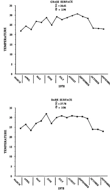
ENVIRONMENTAL VARIABLES.—The recorded temperature values are plotted in Figure 3. The results of a two-way ANOVA with one observation per cell (no replicates were measured for the environmental variables) is shown in Table 2. The hypotheses for differences in mean temperature between stations and with time are both significant at the .05 level, even though the mean temperature at the bare surface is only l°C higher. The minimum at the bare station was 23°C and at the grass station 22°C. The maximum at each was 32°C and 3l°C, respectively. Table 2 shows the mean square for time is higher than for station differences, and, as might be expected, Figure 3 shows summer temperatures were higher than spring and fall.

The recorded salinity values are shown in Figure 4 and the ANOVA results in Table 2. The slightly higher salinities recorded at the bare station were not statistically significant.

Differences with time, however, were highly significant with minimum salinities of 20°/oo and 22°/oo recorded at the bare and grass stations, respectively, in August.

Oxygen measurements are plotted in Figure 5 and ANOVA results are presented in Table 2. Differences between stations

(10)

TABLE 2.—Analysis of variance for chemical variables on bare surface and grass surface.

Variable Temperature

Salinity

Oxygen

PH

Source Sum of

squares df mean

square P(F)

stations time residual stations time residual stations time residual stations time residual

11.77 281.75 8.47

1 16 16 6.62 1 459.62 16

41.38 16 0.39 1 161.39 16

25.26 16 0.06 1 2.98 16 0.55 16

11.77 17.61 0.53 6.62 28.73 2.59 0.39 10.09 1.58 0.06 0.19 0.03

22.24 33.28 2.56 11.11 0.25 6.39 1.77 5.42

0.00 0.00 0.13 0.00 0.63 0.00 0.20 0.00

w

<

06

5

Eh

NH3

PO4

Si

N02

N02 + N 03

stations time residual stations time residual stations time residual stations time residual stations time residual stations time residual

1823.56 248676.53 15053.94 597.94 9405.39 3368.87 9.52 127.32 120.04 117.23 46728.51 2051.49 0.02 0.83 0.15 1424.70 36134.21 36611.80

1 16 16 1 16 16 1 16 16 1 16 16 1 16 16 1 16 16

1823.56 15542.28 940.87 597.94 587.84 210.55 9.52 7.96 7.50 117.23 2920.53 128.22 0.02 0.05 0.01 1424.70 2258.39 2288.24

1.94 16.52 2.84 2.79 1.27 1.06 0.91 22.78 2.25 5.53 0.62 0.99

0.18 0.00 0.11 0.02 0.28 0.45 0.35 0.00 0.15 0.00 0.44 0.51

were not statistically significant, but differences with time were. As expected, there is an inverse relationship with temperature, and generally the oxygen values are higher in the spring and fall. Minimum values occurred at the bare station in May, June, and July, and at the grass station in July.

Values for pH are plotted in Figure 6 and ANOVA results are presented in Table 2. Differences between recorded values between stations were small and not statistically significant.

Differences with time were significant and, like oxygen, the highest values occurred in spring and fall. Minimum values at both stations were 7.5.

Eh values are plotted in Figure 7 and ANOVA results are presented in Table 2. Although the difference in the mean value between stations was relatively large (Figure 7) it was not statistically significant. On the other hand, differences with time were highly significant, and fluctuated greatly between sampling times. Minimum values at the bare station and grass station were -208 and -128 mV, respectively.

NH3 values are plotted in Figure 8 and results of the ANOVA

CRASS SURFACE

£ = 26.61 8 = 2.96

•w

⁴^r

'V V

1978

BARE SURFACE

$ = 27.78 3 = 3.06

1978

» ' V \

FIGURE 3.—Temperature measurements in °C.

are presented in Table 2. No significant difference was observed between stations, but, once again, differences with time were highly significant. Very low to zero values were recorded in the spring and fall with maxima at both stations in the summer.

P0⁴ values are plotted in Figure 9 and ANOVA results are presented in Table 2. No statistical difference was observed between stations or with time. The measured values were generally very low to zero with the exception of the bare station in September which appears to be an outlier.

The measured Si values are plotted in Figure 10 and the ANOVA results are presented in Table 2. No statistical difference was observed between stations, but differences with time were significant. Zero values were recorded at both stations in

(11)

NUMBER 36

3 20

%\ *

GRASS SURFACE

£ =28.79 8 = 3J5

% •%. *** *•>„ % .

GRASS SURFACE

£ = 4.47 C =1.83

% X XI \ X

1978 1978

2 20

<

BARE SURFACE

\X =29.68 O • 4.48

\hr

1978

^

z w 6 rj 6

>

x o

BARE SURFACE ji =4.26 8 = 2.89

•V

i i •• i ^ i - ^ i < ^ 1978

FIGURE 4.—Salinity measurements in %o.

FIGURE 5.—Oxygen measurements in mg-at/1.

(12)

GRASS SURFACE

£ = 8.01 O =0-24

\ \ \ ^

**% \ W i^**

1978

• * . c u kfe>

*> I ^ V °A. <*.

a 8.o

BARE SURFACE ft = 8.10 S =0.41

\ % h

1978 FIGURE 6.—pH measurements.

200 150 100 SO 0

i

•SO

-100 -ISO

-200

GRASS SURFACE

£ = -4.06 0 = 78.29

-250

% % X \\ n

'<& i ^ \

1978

200 150 100 50 0 - -50- -100 -150

BARE SURFACE ji = -18.71 8 = 101.75

4- t>> -fei

^'xi\i\r\

\ i v* i

1978

FIGURE 7.—Eh measurements in mV.

(13)

NUMBER 36

100

80 -

60 -

40

GRASS SURFACE

$ =4.28 6 = 8.0S

18 16 14 12 -I

^ 10

o

GRASS SURFACE

£ =0.54 8 =0.57

1978

BARE SURFACE

£ = 12.67 0 = 27.09

1978

FIGURE 8.—NH3 measurements in ug-at/1.

1978

FIGURE 9.—P04 measurements in ug-at/1.

(14)

53 75

w

GRASS SURFACE

£ = 48.96 8 = 40 32

4s

1978 ** * 0.7 -,

0.6

0.2 -

V %

GRASS SURFACE

£ = 0.14 0 = 0.16

\ *> v rv \

_ij_>

1978 V V \

1 0 0 •

53 75 -

BARE SURFACE

£ = S2.67 6 = 37.73

(1.7

0.2

BARE SURFACE

£ = 0.19 O = 0.19

% *c-„

1978

^

FIGURE 10.—Si measurements in ug-at/1. FIGURE 11.—N02 measurements in ug-at/1.

(15)

NUMBER 36

300 -I

250 •

200

150

100 •

50 -

4

\ ^4r

GRASS SURFACE U = 19.03 3 = 66.28

\ | X \ \

1 \

1978

BARE SURFACE

£ = 6.09 0 = 12.38

1978

FIGURE 12.—N02 + N03 measurements in ug-at/l.

August; however, values generally increase from March to November.

N02 values are plotted in Figure 11 and the ANOVA results are presented in Table 2. Significant differences were again noted only with time. In general, values are low with maxima in summer and fall at the bare station and spring, summer, and fall at the grass station. Both stations had minima values from late August until early October.

N02 + N03 values are plotted in Figure 12, and ANOVA results are presented in Table 2. No significant differences were observed between stations or with time. An unexplainably high value was recorded in April at the grass station.

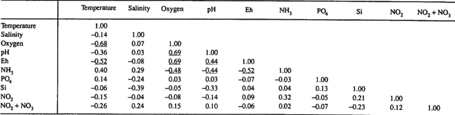
Table 3 shows the correlation coefficients between the environmental variables. Temperature and NH³ are positively correlated with one another and negatively with oxygen, pH, and Eh which are all positively correlated with one another.

Consequently, any hypothesis concerning the significance of a particular variable on species density is not independent of the others.

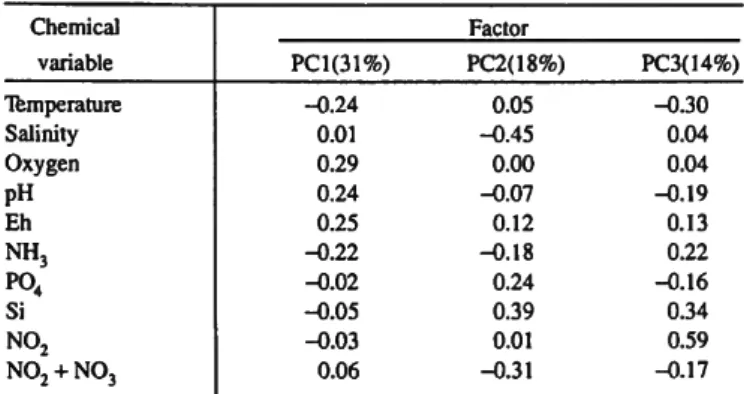
A way to avoid this difficulty is to transform the original variables to principal components. Principal component analysis is a technique which produces a succinct parsimonious summarization of many correlated (non-zero covariance) variables by transforming the original variables to independent (zero covariance) variables called principal components. An additional advantage of the technique is that the first principal component will account for most of the variability in the data, the second less, and so on (Seal, 1964). Eigenvalues were calculated from the correlation matrix (Table 3) using the

SYSTAT statistical package. The first three eigenvectors account for 63.43% of the variability. The factor score coefficients (standardized vectors which when multiplied by the original standardized variables produce the principal components) indicate that all the environmental variables contribute substan- tially to the first three principal components (Table 4). The coefficients (Table 4) indicate that the first principal component (PCI) accounting for 31% of the variability contrasts

TABLE 3.—Correlation matrix for chemical variables for bare surface and grass surface. 0.05 level is underlined.

Temperature Salinity Oxygen pH Eh NH3

P04

Si N02

N02 + N03

Temperature 1.00 -0.14 -0.68 -0.36 -0.52 0.40 0.14 -0.06 -0.15 -0.26

Salinity

1.00 0.07 0.03 -0.08 0.29 -0.24 -0.39 - 0 0 4 0.24

Oxygen

1.00 0.69 0.69 -0.48 0.03 -O.05 -0.08 0.15

PH

1.00 QM -0.44 0.03 -0.33 -0.14 0.10

Eh

1.00 -0.52 -0.07 0.04 0.09 -0.06

NH3

1.00 -0.03 0.04 0.32 0.02

P04

1.00 0.13 -0.05 -0.07

Si

1.00 0.21 -0.23

N02

1.00 0.12

N0² + N 0³

1.00

(16)

10 SMITHSONIAN CONTRIBUTIONS TO THE MARINE SCIENCES TABLE 4.—Factor score coeffecients for chemical variables for bare surface and

grass surface.

Chemical variable Temperature Salinity Oxygen pH Eh NH3

P04

Si N0² N02 + N03

Factor PC 1(31%)

-0.24 0.01 0.29 0.24 0.25 -0.22 -O.02 -0.05 -0.03 0.06

PC2(18%) 0.05 -0.45 0.00 -0.07 0.12 -0.18 0.24 0.39 0.01 -0.31

PC3(14%) -0.30

0.04 0.04 -0.19 0.13 0.22 -0.16 0.34 0.59

^0.17

S IOOO

Z U 100 -:

GRASS SURFACE QUINQUELOCULINA

ji = 254.68 0 = 350.65

**>* rv v** _{«> i x}

2 iooo H 7.

z

K O

z

W 100 -

1978

DARE SURFACE QUINQUELOCULINA

£ =328.59

= 585 .57

* i \ \ • % 1978

temperature and NH3 with oxygen, pH, and Eh. The second principal component (PC2) accounting for 18% of the variability consists mainly of salinity, Si, and N 02 + N03, although P0⁴, NH³, and Eh also contribute and a line of demarkation is not as clear cut as for PCI. The coefficients (Table 4) indicate that the third principal component (PC3) accounting for 14% of the variability consists mainly of N02, Si, and temperature, but again there is no dramatic demarkation. The most highly correlated variables (Table 3) are all concentrated on PC 1.

SPECIES DENSITIES, STATION DIFFERENCES, PERIODICITY, AND ENVIRONMENTAL VARIABLES.—Quinqueloc-

ulina: Quinqueloculina was the most abundant taxon making up about 75% of the total living foraminifera at the surface stations. A plot of the mean densities observed at the bare and grass surface at the two stations is shown in Figure 13.

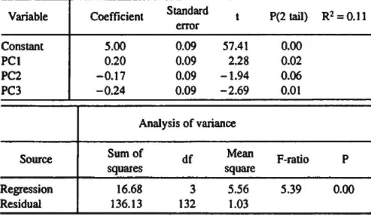
The ANOVA table for six hypotheses is shown in Table 5. We recall that each hypothesis is formulated by equating the desired (3 to zero. For example, the Q. model used to test for station differences deletes B,, for 7i/3 periodicity and interaction P3 = p4 = (i7 = (3g = 0, and so on. Table 5 indicates that all hypotheses except for station differences are significant. The overall mean density at the bare station is higher than at the grass station, but is not statistically significant at the chosen 0.05 level. Figure 13 shows that the bare station had high densities in spring while the grass station had high densities in summer. The environmental variables are significant as a group. Because they are not independent, testing for the significance of each individually is risky. Nevertheless, using the standard errors of the (3's from the co model for calculating confidence limits indicates oxygen, Eh, P04, Si, and N02 + N0³ are significant. Again, emphasizing that the variables are not independent, the ease of calculation using "SYSTAT" made the calculation of simple regressions for each of the variables vs. density irresistible. The results shown in Table 6 indicate the regressions for oxygen, pH, P0⁴, Si, and N0² are significant. A way of avoiding the correlations between variables is to calculate a multiple regression using principal components instead of the original variables. Because the

TABLE 5.—Statistical analysis of GLM for Quinqueloculina for bare surface and grass surface.

FIGURE 13.—Mean number of individuals of Quinqueloculina per 5 ml of sediment (density).

Variability on account of Stations 7t/3 periodicity

and interaction n/6 periodicity

and interaction rc/3 interaction JI/6 interaction Environmental

variables Residual

Sum of squares 1.86 22.53 27.50 9.88 20.45 37.34 59.17

df 1 4 4 2 2 10 116

Mean square 1.86 5.63 6.88 4.94 10.23 3.73 0.51

F 3.64 11.04 13.38 9.68 20.05 7.32

P(F) 0.06 0.00 0.00 0.00 0.00 0.00

(17)

NUMBER 36 11

TABLE 6.—Values of F-ratio's for simple regressions on species densities and environmental variables at bare surface and grass surface. (+ indicates signficant (.05 level) positive value of p; - significant negative value of (J.)

Environmental variables

Temperature Salinity Oxygen PH Eh NH, PO4

Si N02

N02 + NO,

i

0.05 0.20 7.66+

15.44+

0.15 1.64 4.00"

7.23- 4.38"

0.07

5.20- 21.10+

13.22- 16.99+

0.08 0.00 2.03 7.60"

0.05 1.02

/

0.29 5.77+

0.08 0.10 0.08 1.98 1.19 0.25 9.60*

0.22

2.37 49.23+

0.54 0.83 0.41 1.22 11.21+

17.88"

0.67 6.64+

$

/

4.09"

6.79"

4.37+

3.10 0.19 7.09"

1.59 3.36 1.95 0.27

principal components are orthogonal, each hypothesis is independent and the analysis is similar to a one-way ANOVA.

The results of an analysis on the log densities of Quinqueloc- ulina and the first three PC's of the environmental variables are shown in Table 7. The overall F-ratio is significant and the test for the significance of each PC, which are independent, indicates that PCI and PC3 are significant at the 0.05 level while PC2 is nearly so. We recall from Table 4 that temperature, oxygen, pH, Eh, and NH3 all contribute nearly equally to the first PC, and the third PC is weighed heavily on temperature, Si, and N0². Thus, the analysis using principal components requires seven of the 10 environmental variables for two PC's and 10 for three to explain the results. All of the above analyses indicate that the identification of one or two variables as solely significant for the observed densities is impossible.

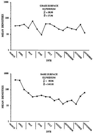
Elphidium: Elphidium constitutes about 14% of the total living population and mean densities at the bare and grass stations are plotted in Figure 14 and the results of the GLM

TABLE 7.—Regression of Quinqueloculina and principal components for bare surface and grass surface.

Variable Constant PCI PC2 PC3

Coefficient 5.00 0.20 -0.17 -0.24

Standard error 0.09 0.09 0.09 0.09

t 57.41

2.28 -1.94 -2.69

P(2 tail) 0.00 0.02 0.06 0.01

R2 = 0.11

Source Regression Residual

Analysis of variance Sum of .r squares

16.68 3 136.13 132

Mean square 5.56 1.03

F-ratio 5.39

P 0.00

analysis is presented in Table 8. Although the mean density at the bare station is again higher than at the grass station, it is not statistically significant. The TC/3 periodicity and interaction hypotheses are significant, but the 7t/6's are not. Figure 14 indicates a spring high at the bare station, but no pronounced summer high at the grass station as was observed with Quinqueloculina. The group of environmental variables are significant, and the p's for Eh, P04, N02, and N 02 + N03 were significant. Regressions of density vs. each individual environmental variable yielded a significant F-ratio for temperature, salinity, oxygen, pH, and Si (Table 6). The results of multiple-regression of Elphidium densities and the first three PC's of the environmental variables are shown in Table 9. The first two PC's are significant and these account for all of the environmental variables except N02. Here, we note that individual tests of the P's from the co model and individual P's from simple regressions do not agree testifying to the difficulty encountered when variables are highly correlated.

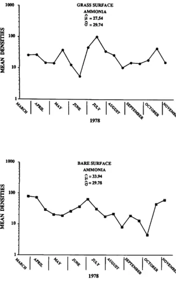
Ammonia: Ammonia makes up about 8% of the total living population and mean densities at the bare and grass stations are plotted in Figure 15. The results of the GLM analysis are presented in Table 10. The overall mean density is slightly higher at the bare station, but not significantly so. The xc/3 periodicity and interaction hypotheses are significant and Figure 15 indicates an early spring maximum at the bare station while both stations have summer and fall maxima. Environ- mental variables are significant as a group and the (3's for Eh, N02, and N02 + N03 were significant. Individual simple regressions on density vs. environmental variables yielded significant F-ratios for salinity and N 0² (Table 6). The results of the multiple regression on densities of Ammonia and the PC's of the environmental variables are shown in Table 11. The results present us with a small dilemma because the F-ratio for the overall analysis has a probability of 0.06 which is slightly above our chosen level, and, therefore, is not significant. On the other hand, PC3 is significant (Table 11). If we choose to regard the third principal component as significant, then temperature, Si, and N02 are the major contributors, especially N02 (Table 4). The F-ratio for environmental variables in the co model, while significant, is the smallest encountered for any of the five taxa analyzed. Ammonia appears, then, to be the least influenced by the 10 variables measured in this study.

Bolivina: Bolivina constitutes about 1% of the total living population and mean densities at the bare and grass stations are plotted in Figure 16. The results of the GLM analysis are shown in Table 12. Although the differences in densities between stations are small, they are, nevertheless, statistically significant, and the highest density is at the grass station. None of the hypotheses for periodicity are significant. There does appear to be a decrease in density over the course of sampling, but the fluctuations in density shown in Figure 16 are small compared to those considered previously (note the difference in the scale of the ordinate). The environmental variables are significant as

(18)

12 SMITHSONIAN CONTRIBUTIONS TO THE MARINE SCIENCES

1000

z

Q

z <

a 10

GRASS SURFACE ELPHIDrUM

£ = 30.90 CT = 17.96

1978

V ^' S

TABLE 8.—Statistical analysis of GLM for Elphidium for bare surface and grass surface.

Variability on account of Stations 7C/3 periodicity

and interaction TC/6 periodicity

and interaction 7t/3 interaction 7t/6 interaction Environmental

variables Residual

Sum of squares 0.88 8.28 2.94 3.73 2.91 28.43 57.04

df 1 4 4 2 2 10 116

Mean square 0.88 2.07 0.74 1.87 1.45 2.84 0.49

F 1.78 4.21 1.49 3.79 2.95 5.78

P(F) 0.18 0.00 0.21 0.03 0.06 0.00

BARE SURFACE ELPHIDIUM

(2= 80.96 a = 14S.S8

1+

1978

FIGURE 14.—Mean number of individuals of Elphidium per 5 ml of sediment (density).

TABLE 9.—Regression of Elphidium and principal components for bare surface and grass surface.

Coefficient 3.50 0.21 -0.30 -0.03

Standard error 0.07 0.07 0.07 0.07

t 50.73

3.05 -4.32 -0.40

P(2 tail) 0.00 0.00 0.00 0.69

R2 = 0.18

Analysis of variance

Sum of .f

squares

18.25 3 85.54 132

Mean square 6.08 0.65

F-ratio 9.39

P 0.00

a group, and the (3's for salinity and Si were significant. F-ratios for simple regressions are significant for salinity, P04, Si, and N0² + N0³ (Table 6). Multiple regression on densities of Bolivina and the first three PC's of the environmental variables are shown in Table 13. Only PC2 consisting mostly of salinity, Si, and N02 + N03 (Table 4) is significant. The relationship with salinity and to a lesser extent with Si are notable for this species.

Ammobaculites: Ammobaculites also constitutes about 1%

of the total living population and mean densities for the bare and grass stations are plotted in Figure 17. The results of the GLM analysis are shown in Table 14. The hypothesis for station differences is significant with the highest densities occurring at the grass surface. The rc/3 periodicity and interaction hypotheses are significant, and Figure 17 indicates the now familiar spring maximum was observed at the bare station after which time the densities remained very low (Appendix 1). At the grass surface the densities increased overall during the sampling duration (Appendix 2). The hypothesis for the environmental variables is significant. The

(3's of the CO model for the variables pH, P04, Si, N02, and N02 + N03 were significant. The F-ratios for temperature, salinity, oxygen, and NH³ were significant for simple regressions on density and environmental variables (Table 6). The results of a multiple regression on the densities of Ammobacu- lites and the first three PC's of the environmental variables are shown in Table 15. The first two PC's are significant indicating that all the variables except for N02 (Table 4) are important contributors. Again, we note the inconsistencies obtained by testing the environmental variables individually.

In summary, we recognize no station differences for the three most abundant taxa. For the rare species Bolivina and Ammobaculites which together constitute only about 2% of the total living population, densities are higher at the grass station.

All of the taxa except for Bolivina exhibited periodicity.

Quinqueloculina, Elphidium, and Ammonia all showed high densities in spring at the bare surface station and in summer at the grass surface. Bolivina exhibited an overall decreasing density from spring onward at both stations while Ammobacu- lites increased at the grass surface station and decreased at the

(19)

NUMBER 36 13

1000

100

V

GRASS SURFACE AMMONIA ji = 27 £4 O = 29.74

*A \ \

x I %

1978 %

TABLE 10.—Statistical analysis of GLM for Ammonia for bare surface and grass surface.

Variability on account of Stations JI/3 periodicity

and interaction rt/6 periodicity

and interaction 7i/3 interaction n/6 interaction Environmental

variables Residual

Sum of squares 0.06 11.29 4.24 6.38 1.94 16.60 54.70

df 1 4 4 2 2 10 116

Mean square

0.06 2.82 1.06 3.19 0.97 1.66 0.47

F 0.13 5.98 2.24 6.76 2.05 3.52

p(F) 0.72 0.00 0.07 0.00 0.13 0.00

B A R E S U R F A C E A M M O N I A

1 = 33.94 ]i-

•• 29.78

M \ *>

1978

<K I ' A

FIGURE 15.—Mean number of individuals of Ammonia per 5 ml of sediment (density).

TABLE 11.—Regression of Ammonia and principal components for bare surface and grass surface.

Coefficient 3.14 -0.01 -0.12 0.15

Standard error 0.07 0.07 0.07 0.07

t 45.92 -0.16 -1.72 2.18

P(2 tail) 0.00 0.87 0.09 0.03

R2 = 0.06

Analysis of variance

Sum of .f

squares

4.92 3 83.81 132

Mean square

1.64 0.64

F-ratio 2.58

P 0.06

bare surface. The environmental variables were significant as a group for all taxa, however, individual variables cannot be evaluated with confidence.

Grass Surface and Grass 10 cm

ENVIRONMENTAL VARIABLES.—The recorded temperature values are plotted in Figure 18, and the results of a two-way ANOVA testing for differences between surface and 10 cm and with time are shown for temperature and all the other environmental variables in Table 16. The hypothesis testing for differences in mean temperature between the surface and 10 cm depth is not significant, however, the hypothesis testing for time is. As everyone knows, the water is warmer in the summer and cooler in spring and fall. A very high temperature was recorded in June and a very low one in August at 10 cm.

The measured salinity values are shown in Figure 19. Only the hypothesis for time is significant. Salinities were highest in

spring except for the first observation in March at 10 cm. Both stations experienced a dip in salinity in August.

The recorded oxygen values are shown in Figure 20. The mean square for differences between surface and 10 cm is large and highly significant, and the mean square for time, although relatively much smaller, is nearly significant. Figure 20 illustrates and Appendix 6 tabulates zero recordings for oxygen during spring and summer at 10 cm making the difference between the surface and 10 cm (depth hypothesis) so dramatic.

The measured pH values are plotted in Figure 21. The depth hypothesis is significant, and the pH is always lower at 10 cm (Figure 21, Appendix 5, 6). Even at 10 cm, however, only one reading (November) recorded a value below 7.

Eh values are plotted in Figure 22. The depth hypothesis is significant. Values of Eh at 10 cm are always negative, and usually highly so, while the values at the surface fluctuate from positive to negative with a slightly negative mean (Figure 22, Appendix 5, 6).

(20)

14 SMITHSONIAN CONTRIBUTIONS TO THE MARINE SCIENCES

GRASS SURFACE BOLIVINA

V = 7.26 S = 7.98

•fe.

A

I \ I %

1978

TABLE 12.—Statistical analysis of GLM for Bolivina for bare surface and grass surface.

Variability on account of Stations TC/3 periodicity

and interaction TC/6 periodicity

and interaction

;r./3 interaction 7C/6 interaction Environmental

variables Residual

Sum of squares 4.03 4.38 3.33 1.25 0.36 42.21 62.77

df 1 4 4 2 2 10 116

Mean square 4.03 1.09 0.83 0.62 0.18 4.22 0.54

F 7.45 2.02 1.54 1.15 0.33 7.80

P(F) 0.01 0.10 0.20 0.32 0.72 0.00

•if 1*

w

BARE SURFACE BOLIVINA

(1 = 3.38 8 = 3.82

V>>

1978

FIGURE 16.—Mean number of individuals of Bolivina per 5 ml of sediment (density).

TABLE 13.—Regression of Bolivina and principal components for bare surface and grass surface.

Coefficient 1.38 0.04 -0.52 0.01

Standard error 0.07 0.07 0.07 0.07

t 19.10

0.47 -7.14 0.19

P(2 tail) 0.00 0.64 0.00 0.85

R² = 0.28

Analysis of variance Sum of .r squares

36.34 3 93.66 132

Mean square 12.11

0.71

F-ratio 17.07

P 0.00

NH3 values are plotted in Figure 23. The depth hypothesis is significant. The values at 10 cm are usually two orders of magnitude greater than at the surface (Appendix 5, 6). Two zero values were recorded at 10 cm, one in April and one in October. We suspect these anomalies are due to problems with instrumentation.

P04 values are plotted in Figure 24. The hypothesis for depth is significant. The values for P04 were very low at the surface, and one or two orders of magnitude higher at 10 cm (Appendix 5, 6). A very high value was recorded at 10 cm in June.

Si values are plotted in Figure 25 and the hypothesis for depth is significant. The values for Si at the surface are an order of magnitude smaller than at 10 cm (Appendix 5, 6). At 10 cm zero values were recorded in April, August, and October.

Except for the zero value in August, the pattern is very similar to that observed for NH³ at 10 cm.

N 0² values are plotted in Figure 26. The hypothesis for depth is significant, and values for N02 are low. At 10 cm very low values were recorded in all months except October.

N02 + N03 values are plotted in Figure 27. There is no significant difference with depth or with time. Except for one measurement at the surface in April (Figure 27, Appendix 5) all the measurements were low.

The two-way ANOVA's for environmental variables at the bare surface vs. grass surface showed most significant differences are with time (Table 2). In contrast, the analysis for grass surface vs. grass 10 cm shows most of the significant differences are with depth (Table 16). Moreover, the F-ratios for the latter are usually much higher. We have, then, a situation where, except for temperature, salinity, and N02 + N03, there are much larger differences than at the surface stations.

The environmental variables are highly correlated as shown in Table 17. High positive values occur between oxygen and Eh, oxygen and N0², pH and Eh, Eh and N0², NH³ and P0⁴, NH3 and Si, and P04 and Si. High negative values occur between oxygen and NH³, oxygen and P0⁴, oxygen and Si, pH and NH3, pH and Si, Eh and NH3, Eh and P04, and Eh and Si.