FOREIGN EXCHANGE MARKET PRESSURE, EXCHANGE RATE AND TRADE BALANCE IN NIGERIA: IS THERE EVIDENCE OF THE J-CURVE
EFFECT?
David Terfa Akighir*1
1 Department of Economics, Benue State University Makurdi, Makurdi, Nigeria
ABSTRACT
The paper examined the relationship between the pressure in the exchange market, exchange rate, and trade balance in Nigeria to ascertain whether or not the J-Curve effects exist. The investigation was anchored on the Marshal- Lerner and the J-Curve theories using annual time series data from 1986 to 2021. The Structural Vector Autoregressive (SVAR) technique was employed, and the findings revealed that the pressure in the exchange market exerts a strong contemporaneous positive effect on the exchange rate in the country.
Also, the findings showed that the exchange rate has a strong contemporaneous negative effect on the trade balance. Furthermore, the long-run results indicated that the exchange rate has a positive but weak effect on the country’s trade balance. Based on these findings, it was concluded that the relationship that exists among foreign exchange market pressure, exchange rate, and balance of trade suggests the potentiality of the J-Curve effects in the economy. The study recommended that local production of goods and services in Nigeria should be strengthened so that the depreciation of the naira would improve the trade balance. In the event of naira depreciation, domestic consumers could redirect their demand to the consumption of locally produced goods and services. Also, local production, especially in manufacturing and agricultural processing, should be encouraged, and the quality of the products be enhanced for competitive exportation to improve the trade balance in the country. The policy implication is that policymakers can leverage naira depreciation as a policy tool to enhance Nigeria’s balance of trade.
Keywords: Exchange Rate, Foreign Exchange Market Pressure, J-Curve, Trade Balance, Structural Vector Autoregressive
JEL: F; F1; F31; F32
To cite this document: Akighir, D. T. (2023). Foreign Exchange Market Pressure, Exchange Rate, and Trade Balance in Nigeria: Is There Evidence of The J-Curve Effect?. JDE (Journal of Developing Economies), 8(2), 340-363. https://doi.org/10.20473/jde.v8i2.44656
Introduction
Trade balance, also called the balance of trade, is the differential between a country’s monetary value of its imports and exports over a given period. Exchange rate dynamics are critical in influencing an economy’s trade balance position. According to Jain et al. (2023), export-oriented economies (economies with trade surpluses) can manage exchange rates to their advantage. Currency depreciation affects countries’ trade balance differently depending on the elasticities of the supply of exports and imports of an economy (Cheng, 2020). Because
ARTICLE INFO
Received: April 6th, 2023 Revised: May 11th, 2023 Accepted: June 7th, 2023 Online: December 3rd, 2023
*Correspondence:
David terfa Akighir
E-mail: akighirdavidterfa@gmail.com
JDE (Journal of Developing Economies) p-ISSN: 2541-1012; e-ISSN: 2528-2018 DOI: 10.20473/jde.v8i2.44656
of this, the Marshall-Lerner condition stipulates that, given the elasticities of the supply of exports and imports of goods with infinite response and the trade balance in the initial period, the aggregate of these elasticities in terms of the absolute values should be higher than unity for currency depreciation to increase the trade balance of an economy. Also, when this sum is less than unity, depreciation will make the trade balance unfavorable (Obadan, 2012).
Furthermore, when the imports of an economy are higher than its exports, it exerts pressure on the exchange rate. This is because a decline in export revenue affects Apex Bank’s ability to manage the exchange rate effectively. When the Apex Bank of an economy is faced with the inability to manage the exchange rate due to reduced external reserves, there would be depreciation of the domestic currency given a surge in demand for the available scarce foreign exchange by the economic agents (Central Bank of Nigeria (CBN), 2016). Again, when the demand for foreign exchange exceeds its supply in an economy due to excessive imports over exports, it creates pressure in the exchange market. The foreign exchange market pressure then depreciates the affected economy’s currency, making imports costly and exports cheaper (Kpoghul et al., 2022). According to Akbostanci (2002), domestic currency depreciation is supposed to improve the competitiveness of local products in the international market in the future based on the postulations of the J-Curve theory.
The Nigerian economy has faced an intense foreign exchange crisis over the years. This has posed a lot of challenges to the effective exchange market management of the economy.
As a result, the exchange rate has depreciated unabated in the country (Ominyi et al., 2020).
Available data from the CBN (2022) reveal that the real effective exchange rate increased from 69.20% in 1999 to 109.5% in 2021, representing a 36.80% increase over the years. Based on the J-Curve theory’s theoretical expositions, this naira depreciation is supposed to galvanize long-run trade surplus for the Nigerian economy. However, the historical data of Nigeria’s trade balance have fluctuated over the years. In 1999, the trade balance witnessed a surplus of $4.87 billion, which rose to $16.01 billion in 2000; it again declined to $5.05 billion in 2001.
It marginally increased to $6.15 billion in 2002 and then dipped to $4.37 billion in 2003. It rose from $11.75 billion in 2004, maintained a surplus position, and fluctuated between 2007 and 2009. By 2012, it stood at $84.54 billion and declined to $32.72 billion in 2014, after which it assumed a deficit position from 2015 to 2020 (National Bureau of Statistics (NBS), 2021).
NBS (2021) report on Foreign Trade in Goods Statistics that further revealed that Nigeria’s balance of trade rose significantly from a deficit of $327 billion recorded in the previous quarter to $1.1 billion in the fourth quarter of 2021; when compared to the corresponding period of the previous year. It has increased by 115% from the $7.57 billion deficit recorded in the fourth quarter of 2020. Overall, the aggregate trade balance for 2021 remains in deficit to the tune of $6.49 billion, though better than the $21.37 billion recorded in 2020.
Given this sustained exchange rate depreciation amid the fluctuating trade balance in the country, it is difficult to establish whether or not the trade balance has positively responded to exchange rate depreciation in the country in line with the postulations of the J-Curve theory. Previous studies investigating this relationship in the country have presented mixed conclusions on the subject. For example, previous studies such as: (Usman & Bukar, 2020; Andohol, 2020; Sani et al., 2019; Gatawa et al, 2018; Olanipekun & Ogunsola, 2017), among others have used various methodologies and have established that exchange rate depreciation has not improved balance of trade in Nigeria. On the other hand, earlier studies by (David & Elijah, 2020; Odili, 2014) have established that domestic currency depreciation in Nigeria increases the economy’s trade balance. Also, Akpansung (2021) used the ARDL model
and found that exchange rate depreciation exerts a significant positive impact on the trade balance in the short-run but an insignificant negative effect in the long-run.
Given these divergent arguments, the impact of exchange rate depreciation on trade balance in Nigeria is empirically not clear; this has serious economic policy implications for exchange rate management in the economy. Thus, understanding the impact of naira depreciation on the balance of trade in the country is imperative. This is important because of the economy’s underdeveloped financial systems and persistent trade balance deficit.
Given these economic attributes, if naira depreciation affects the trade balance negatively, policymakers will need to use fiscal and monetary policy prescriptions to stabilize the value of the naira. However, if depreciation improves the trade balance, policymakers can leverage naira depreciation to stimulate exports for sound macroeconomic performance.
The current study has explored the dynamics among foreign exchange market pressure, exchange rate, and trade balance following the postulations of the Marshall-Lerner and the J-Curve theories. This would help affirm or repute empirically the theoretical conditions that indicate the attainment of the J-Curve effects in the case of the Nigerian economy. Second, considering these opposing findings regarding the impact of naira depreciation on the economy, this study has used the real effective exchange rate, which is a composite of the basket of foreign currencies of many trading partners of Nigeria, as opposed to the use of nominal exchange rate by most previous studies. The use of the real effective exchange rate is deemed most appropriate since it is the indicator of the international competitiveness of a nation’s trade compared with its trade partners.
Thus, this study aims to investigate the impact of foreign exchange market pressure on trade balance via exchange rate using the Structural Vector Autoregressive (SVAR). The preference of the SVAR over other techniques is due to its advantages: First, the SVAR can show the transmission mechanism of foreign exchange market pressure to trade balance via the exchange rate. Second, it generates the contemporaneous matrix that helps analyze the short-run dynamic impact of exchange rate on trade balance as postulated by the J-Curve hypothesis. Again, the SVAR generates forecast toolkits, namely, the impulse response graphs and the variance decompositions tables that can immensely assist in analyzing the dynamic short and long-run responses of the trade balance to innovations in foreign exchange market pressure and the dynamics in the exchange rate in the economy.
Therefore, this study has two novelties and two contributions. First, it used the real effective exchange rate to capture the exchange rate dynamics of other trading partners of Nigeria. Second, it used the SVAR as the most appropriate analytical tool to ascertain the intertemporal dynamics among Nigeria’s foreign exchange market pressure, exchange rate, and trade balance. Given this uniqueness, the study has immense policy potency to the Nigerian economy in that the findings of the study provide a policy prescription of leveraging the naira depreciation as a veritable policy option to enhance the balance of trade of the Nigerian economy, an import-dependent economy facing persistent trade deficit amid naira depreciation. The rest of this paper is organized in the following sections after the introduction:
The literature review is presented in section two; data and research methods are presented in section three; section four dwells on stylized facts; section five depicts the results; while section six is on conclusion and policy recommendations.
Literature Review Conceptual Clarification
Conceptually, the CBN (2016) has defined foreign exchange market pressure (EMP) as disequilibrium in the exchange market that is associated with currency depreciation in an economy operating a floating exchange rate regime. It is an index that has to do with the movements in international reserves, the nominal exchange rate, and, in some cases, the level of money supply in an economy.
Furthermore, Gilal & Mahesar (2016) conceptualized the pressure in the exchange market as a situation where the demand for domestic currency is higher than its supply in an economy. Excess demand for domestic currency in the foreign exchange market precipitates domestic currency appreciation against the foreign currency. Lower demand for domestic currency precipitates local currency depreciation, thereby losing its value against foreign currency. In this study, this pressure is defined as the disequilibrium in the foreign exchange market, which causes excess demand for or supply of foreign exchange to exert undesirable effects on the exchange rate and other key macroeconomic trajectories, making the monetary authorities decide to defend the domestic currency.
The World Bank (2022a) conceptualized the exchange rate as a rate at which one currency is exchanged for another. In other words, it is the value that a currency is converted to another currency to affect international transactions. This study uses the Real Effective Exchange Rate (REER). Accordingly, the International Monetary Fund (IMF) (2020) defined the REER as the weighted average of a country’s currency in relation to an index or basket of other major currencies deflated by the price, which indicates the exports and imports competitiveness of a nation with the rest of the world.
Again, the concept of balance of trade has been defined as the differential of the monetary values of exports and imports of an economy. The computation of the balance of trade reveals either positive or negative outcomes. A positive trade balance (surplus) implies the excess of exports over imports, and a negative trade balance (deficit) implies the excess of imports over exports (Obadan, 2012).
Theoretical Background
Theoretically, this study is hinged on the Marshall-Lerner and J-Curve theories’
theoretical foundations. The Marshall-Lerner (M-L) theory was put forth by A. Marshall in 1923 and A. Lerner in 1944 to analyze the dynamics of excess demand for foreign currencies over its supply that depreciates the currency of the affected economy under a floating exchange rate regime with its attendant consequences on the trade balance. It posits that currency depreciation changes the relative prices of locally produced and foreign goods, negatively affecting an economy’s trade balance (Crocket, 1987).
Thus, the M-L theory stipulates that, given the elasticities of the supply of exports and imports of goods with infinite response and the trade balance in the initial period, the aggregate of these elasticities in terms of the absolute values should be higher than unity for currency depreciation to increase the trade balance of an economy. When the total of these elasticities is less than one, depreciation will adversely affect the trade balance. If the summation of the elasticities is precisely one, depreciation will not affect the trade balance.
Therefore, it is only when this condition is satisfied that a change in exchange rate changes can exert the expected effects on the balance of trade; that is, it will increase the trade balance of
the country experiencing currency depreciation and weaken the trade balance of the country experiencing currency appreciation (Kulkarni & Clarke, 2009). In the context of a change in the trade balance, the Marshall-Lerner condition is expressed as follows: DB=dX e( X+eM-1) Where: DB changes in the balance of trade, d = devaluation rate, X the exports of goods and services denominated in the value of currency broad, eM the responsiveness of local demand to imported goods abroad, eX the responsiveness of international demand to a local country’s export of goods (Obadan, 2012).
On the other hand, the J-Curve theory is associated with the work of Magee (1973), which attempts to provide an analytical exposition of how exchange rate dynamics impact a country’s balance of trade. That is, how a country’s currency depreciation affects the trade balance. It gives a time lag description of how currency depreciation increases trade balance in the long-run (Kulkarni & Clarke, 2009). According to the postulations of the J-Curve theory, currency devaluation or depreciation will make imports costly and exports cheaper; this will cause the current account of the depreciating country to decline. This is because, after currency depreciation, there will be a lag in changing the consumption levels of imported goods. The demand for expensive imports and the demand for cheaper exported goods will subsist in the short-run since consumers of the expensive imported goods will be exploring cheaper substitutes, while the consumers of the cheaper exported goods will adjust their absorption capacity to accommodate the supply of these goods (Doroodian & Roy, 1999).
The J-Curve theory posits that, following the currency depreciation, in the long-run, consumers in the currency-depreciating country will redirect their demand to the consumption of cheaper locally produced goods, while foreign traders, on the other hand, will increase the purchase of goods exported to their economies at relatively lower prices due to the weakened currency value. At this point, the country whose currency depreciated will experience an improved current account balance. Thus, the short-run and long-run trade balance positions during currency depreciation constitute the J-Curve effect (Anju & Uma, 2006). According to Kulkarni & Clarke (2009), if the responsiveness of imports and exports to the price variations is robust enough to signal a significant effect, then the M-L condition will be satisfied for depreciation to exert a long-run impact on the trade balance.
Empirical Review
In terms of previous studies, some studies have analyzed the relationship between foreign exchange market pressure and exchange rate on the one hand and the nexus between exchange rate dynamics and balance of trade in different economies on the other hand. For instance, Wang et al. (2023) used the connectedness network methodology in investigating the spillovers of policy uncertainty to the volatility of exchange rates in a panel of twenty- one economies. The monthly data spanning from 1997 to 2022 was utilized. The study found that the contagious effect of volatility in the exchange rate on policy uncertainty is stronger than the contagious effects exerted by policy uncertainty on exchange rate volatility. Also, the contagious effect of policy uncertainty on exchange rate volatility is majorly found in exchange markets of developing economies.
Furthermore, the findings revealed a higher responsiveness rate of exchange markets of developing economies to perturbations in global shocks. Again, findings indicated that the spillover risks from policy uncertainty to exchange rate volatility occur via a transmission channel. An increase in global economic policy uncertainties gives rise to global exchange rate volatility, further increasing pressure on the exchange markets of developing economies.
Similarly, Huynh et al. (2023) studied the nexus between the directional spillover and connectedness for return and volatility in 9 U.S. dollar exchange rates, which are the most globally traded currencies, and the study focused on the role of trade policy uncertainty. The study utilized monthly data from December 1993 to July 2019. The study’s findings revealed asymmetric spillovers and connectedness among the used exchange rates in the presence of trade policy uncertainty. Also, the study found that the volatility spillover is more influential than the return connectedness between exchange rate and trade policy uncertainty. Relatedly, Olanipekun et al. (2019) investigated the effect of uncertainty on pressure in the exchange market using a sample of twenty economies. The study used quarterly data from 2003Q1 to 2017Q4 and found that increases in uncertainty, inflation, trade, and financial openness tend to increase pressure in the exchange market in the future. Also, GDP, domestic credit, and FDI tend to reduce the pressure regardless of the exchange rate regime. The implication is that an upsurge in this pressure precipitates exchange rate depreciation in an economy.
Furthermore, Ajmal & Arabi (2021) studied the nexus between foreign exchange market pressure and monetary policy in Afghanistan using quarterly data from 2000Q1 to 2019Q4. The paper utilized the Autoregressive Distributed lag model, and findings revealed that foreign reserves, domestic credit contraction, and political uncertainty affect the pressure in the exchange market contemporaneously and in the future period, and consequently, the exchange rate. Also, the study by Kpoghul et al. (2022) x-rayed the nexus among global economic policy uncertainties, foreign capital inflow, and foreign exchange market pressure in Nigeria using Quantiles causality tests and SVAR methodologies. Findings revealed that global economic policy uncertainties granger cause foreign exchange market pressure in Nigeria and economic policy uncertainties affect EMP in Nigeria via foreign capital inflow channels.
Again, Oguzhan et al. (2020) revisited the discourse on the asymmetric impacts of the exchange market pressure on inflation, interest rate, and foreign trade balance in Eastern Europe using the Qualitative VAR models. The study found that an increase/decrease in the foreign exchange market affects inflation and trade balance in the Czech Republic and Poland because of the importation of raw materials for local production. Aboobucker et al. (2021) investigated the relationship between the exchange rate and trade balance in Sri Lanka using the ARDL and Granger causality tests. The study’s findings have revealed that the exchange rate has an inverse long-run relationship with trade balance, and the exchange rate coefficient is higher than unity, which supports the Marshal-Lerner condition. Also, Nusair (2017) used a non-linear ARDL model to verify the existence or otherwise of the J-Curve in 16 European countries. The study found empirical evidence of the J-Curve effects in 12 out of the 16 economies investigated.
Furthermore, Bahmani-Oskooe et al. (2018) employed the non-linear ARDL model on China’s data and her 21 trade partners. They found evidence of J-Curve due to the depreciation of the Yuan. Again, Mwito & Luvanda (2021) used panel linear and non-linear ARDL framework on Kenyan bilateral trade data from 2006Q1 to 2018Q4 and found J-Curve effects in only seven bilateral relations in the context of the symmetric exchange rate. However, 13 cases of the J-Curve effects were evident in the context of the asymmetric exchange rate.
In Nigeria, Akpansung (2021) used the ARDL bounds testing on the Nigerian data for the period of 1986-2019 and found that overall, naira depreciation cannot enhance the trade balance in Nigeria, given its insignificant adverse effects on trade balance in the future and its significant positive contemporaneous effect on trade balance. Also, Andohol (2020) investigated the existence of J-Curve in Nigeria using structural breaks. The study employed
Linear Autoregressive Distributed lag (ARDL) and Non-linear Autoregressive Distributed lag (NARDL) models. The study did not find the existence of a J-Curve but the existence of a reversed J-Curve in Nigeria. Similarly, Sanni et al. (2019); Olanipekun & Ogunsola (2017);
Usman & Bukar (2020) found inverse nexus between naira depreciation and the balance of trade in the economy.
Conversely, Odili (2014) employed the ARDL framework on the Nigerian data from 1971 to 2012 and found a positive and statistically significant relationship between exchange rate and trade balance in the short-run but a positive and insignificant relationship in the long-run. In the same vein, David & Elijah (2020) used the ARDL methodology on the Nigerian data from 1986 to 2018 and found strong positive effects both contemporaneously and in the future. Okafor (2012) evaluated Nigeria’s dynamics of foreign exchange demand for twenty- four years (1986 – 2009). Using the OLS technique, the results revealed that imports drive the surge in foreign exchange demand and not exchange rates.
The findings of the reviewed empirical studies, especially on the Nigerian economy, are divergent. These divergences may, in part, be due to the usage of the nominal exchange rate in literature by previous studies. This study is different from the previous studies, especially in the context of the Nigerian economy, in that it has used the effective exchange rate that considers a basket of foreign currencies that the trading partners use. Also, it has used the foreign exchange market pressure as a predictor of exchange rate depreciation to systematically explore the transmission mechanism to trade balance via the instrumentality of the exchange rate. Lastly, the current research has employed the SVAR model as a hybrid methodology to trace the transmission effect.
Data and Research Methods
The study utilized annual time series data from various issues of the Central Bank of Nigeria (CBN) statistical bulletins, National Bureau of Statistics (NBS) reports, and World Bank trade statistics. The data collected span from 1986 to 2021. The choice of 1986 is predicated upon the premise that this was when the exchange rate was liberalized in the country. To capture the transmission mechanism of the foreign exchange market pressure to trade balance to ascertain whether or not the J-Curve effect exists, the SVAR was specified. The choice of the SVAR amid the array of competing techniques is because the SVAR can show transmission effect and offers the opportunity to estimate impulse response and variance decompositions to analyze shocks among the series. The general form of the SVAR model is written as:
A Z0 t=A Z1 t-1+f1 (1) Where A.O. = the short-run contemporaneous matrix
Zt = the dependent variables vector matrix A1 = the lagged matrix of the dependent variables
Zt-1 = the vector matrix of lagged values of the dependent variables and = the vector matrix of the error terms in the SVAR.
According to the Marshall-Lerner hypothesis, a surge in foreign exchange demand, given its supply, will depreciate the exchange rate with its attendant consequences on the trade balance. Again, The J-Curve hypothesis stipulates that the depreciation of a currency
will cause the trade balance to decline in the immediate period but increase in the future.
Therefore, this transmission can be expressed as follows:
EMP-"EXCH."BOT .- (2)
The study used the two-component index for its computation, where EMP is foreign exchange market pressure. The choice of this component stems from the fact that in Nigeria, the foreign reserves are usually depleted to defend the naira in the event of a crisis in the market. Thus, this component captures the percentage depreciation of the exchange rate and the percentage losses in foreign reserves. The two-component index is computed as follows:
EMP EEE
RRR
100 100
t t
t t
t
t t
1 1
1
= - + - 1
- -
-
b l b - l (3)
Where EMPt is Exchange Market Pressure, Et is Nominal Exchange Rate against USD, Et-1 is one period lag of exchange rate, Rt is the foreign reserves, and Rt-1 is one period lag of foreign reserves (Ammar, 2019). EXCH is the real effective exchange rate index, the weighted average of several currencies against a country’s currency divided by a denominator called the price deflator, and BOT is the balance of trade. The BOT is computed as BOT = the monetary value of Exports Less the monetary value of Imports.
The transposition of the transmission mechanism stated in equation 2 has produced the following models:
( , , , , )
BOTt=f BOT EXCHt-1 t-1EMP EXCH EMPt-1 t t (4)
( , , , , )
EXCHt=f BOT EXCHt-1 t-1 EMP BOT EMPt-1 t t (5)
( , , , , )
EMPt=f BOT EXCHt-1 t-1EMP BOT EXCHt-1 t t (6) Therefore, the normalized equations of the SVAR (1) are further expressed as:
BOTt 111BOTt EXCHt EMPt EXCHt EMPt t 1 121
1 131
1 120
130
a a a a a f1
= - + - + - + + + (7)
EXCHt 211 BOTt EXCHt EMPt BOTt EMPt t 1 221
1 231
1 210
230
a a a a a f2
= - + - + - + + + (8)
EMPt 311 BOTt EXCHt EMPt BOTt EXCHt t 1 321
1 331
1 310
320
a a a a a f3
= - + - + - + + + (9)
The variables in the current values represent the contemporaneous effects. Therefore, by collecting the like terms gives the following expressions:
BOTt 120EXCHt EMPt BOTt EXCHt EMPt t 130
111
1 121
1 131
1 1
a a a a a f
- - = - + - + - + (10)
BOTt EXCHt EMPt BOTt EXCHt EMPt t 210
230
121
1 122
1 231
1 2
a a a a a f
- + - = - + - + - + (11)
BOTt EXCHt EMPt BOTt EXCHt EMPt t 310
320
131
1 132
1 331
1 3
a a a a a f
- - + = - + - + - + (12)
Expressing equations 10 to 12 in matrix form has produced the following:
BOT EXCH
EMP
BOT EXCH
EMP 1
1 1
t t t
t t t
t t t 21
0
31 0
12 0
32 0
13 0
23 0
11 1
21 1
31 1
12 1
22 1
32 1
13 1
23 1
33 1
1 1 1
1 2 3
a a
a a
a a
a a a
a a a
a a a
f f f -
- - -
-
- = +
- - -
R
T SSSS SSSSS
R
T SSSS SSSSS
R
T SSSS SSSSS
R
T SSSS SSSSS
R
T SSSS SSSSS V
X WWWW WWWWW
V
X WWWW WWWWW
V
X WWWW WWWWW
V
X WWWW WWWWW
V
X WWWW WWWWW
(13)
Hence,
A Z0 t=A Z1 t-1+f1 (14) Where A.O. = the short-term effects matrix of the dependent variables
Zt = the column matrix of the dependent variables
A1 = the matrix of the one-period lags of the dependent variables
Zt-1 = the column matrix of the one-period lags of the dependent variables and
ε1t = the column matrix of the stochastic errors.
Model 13 is stated in an over-parameterized form; given its over-parametrization status, the SVAR cannot be invoked. Thus, the recursive technique was followed to place some restrictions on the elements of the upper diagonal of matrix A0 in equation 13 to overcome the challenge of model identification. Therefore, the elements above the main diagonal were set to zero
0
230 130
120 =− =− =
−α α α To produce the parsimonious version of the SVAR as follows:
A
BOT EXCH
EMP
1 0
1 0 0 1
t t t
t t t
0 210
310
320
1 2 3
?
? ?
f f f
= -
- -
= R
T SSSS SSSS
R T SSSS SSSS
R T SSSS SSSS V
X WWWW WWWW
V X WWWW WWWW
V X WWWW WWWW
(15) Where ft=bht, and
0 0
0 0
0 0
12 22
32
b d
d d
= R T SSSS SSSS
V X WWWW
WWWW = Variance one, that is, Var(ηt)=1 A
BOT EXCH
EMP
BOT
EXCH
EMP
1 0
1 0 0 1
0 0
0 0
0 0
t t t
tBOT tEXCH
tEMP
0 210
310 320
12
22
32
a a a
d
d
d
n n
n
= -
- -
= R
T SSSS SSSS
R T SSSS SSSS
R T SSSS SSSS
R T SSSS SSSS V
X WWWW WWWW
V X WWWW WWWW
V X WWWW WWWW
V X WWWW WWWW
(16)
Now, the normalized version of the SVAR defined as:AOZt = A1Zt−1+εt has reduced to the form: A eo t=bht, and bht=bnt. Therefore, the reduced form model to be estimated is expressed as follows:
A eo t=bnt (17)
Where A.O. = the contemporaneous effects short-run 3 X 3 matrix et = the column matrix of stochastic errors in the SVAR
β = the matrix of the innovations in the SVAR and μt = the column matrix of the innovations in the SVAR.
Now, the matrix ‘S’ is stated as:
e A
e BOT e EXCH
e EMP
1 0
1 0 0 1
t o t
t t
t
tBOT t EXCH
tEMP 210
310 320
bn a
a a
n n
n
= = = -
- -
R T SSSS SSSS
R T SSSS SSSS
R T SSSS SSSS V
X WWWW WWWW
V X WWWW WWWW
V X WWWW
WWWW (18)
Finally, the impulse response and variance decomposition functions were estimated to analyze the intertemporal dynamics among the series.
Finding and Discussion
Stylized Facts on Foreign Exchange Market Pressure, Exchange Rate Dynamics, and Balance of Trade in Nigeria
This sub-section presents stylized facts on foreign exchange market pressure, exchange rate, and balance of trade in Nigeria. The episodes of foreign exchange market pressure are presented in the following figure.
Figure 1: Exchange Market Pressure in Nigeria using a 2-Component
The figure reveals the trends of the pressure index in the exchange market, which was computed using the 2-component model from 2000Q1 to 2020Q4. It is evident from the figure that the exchange market has experienced various major episodes of pressure over this period under review. The first episode was between 2000 and 2001. Another major episode was noticed from the first quarter of 2002 through the first quarter of 2003.
Furthermore, the most serious pressure episode was between 2008 and 2009. This period coincided with the global financial crisis caused by the subprime mortgage crisis and the subsequent bankruptcy of the Lehman Brothers in September 2008. As a result, developing countries like Nigeria, which depended on exporting crude oil for foreign exchange, were adversely affected. Similarly, the figure depicts another fundamental pressure episode between 2014 and 2016. This period coincided with the epoch of the slump in global commodity prices, which affected oil prices the most. Nigeria has been a monolithic economy that depends on oil for about 70% of its resources; foreign exchange has worsened, and the economy has even gone into a recession.
Finally, another serious pressure episode was found from quarter four of 2019 through quarter four of 2020. This period coincided with the COVID-19 pandemic era, when the entire global economy was in economic turmoil as a result of the outbreak of the pandemic. The global lockdowns truncated economic activities, and economies of the world were adversely
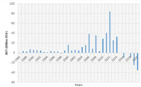
Furthermore, the real effective exchange rate trends in Nigeria from 1986 to 2021 are presented in Figure 2.
Figure 2: Real Effective Exchange Rate in Nigeria from 1986 to 2021
Source: International Monetary Fund (IMF) (2022)
Figure 2 shows the trend of the real effective exchange rate index (2010 = 100) in Nigeria from 1986 to 2021. It is clear from the figure that the real effective exchange rate in Nigeria has fluctuated significantly over the years. It exhibited a sustained increasing trend from 2002 to 2021. It had a maximum value of 273.01 in 1998 and a minimum value of 49.75 in 1992. The minimum value in 1992 may be ascribed to the performance of the monetary policy in 1992, which the Central Bank of Nigeria introduced that improved the overall economic performance of the country at that time, while the surge in the real effective exchange rate in 1998 may be due to the wide differential in the official and black market rates caused by the upsurge in the demand for foreign exchange in the country that time which necessitated the re-introduction of the retail Dutch Auction System (rDAS) in 2002 and the wholesale Dutch Auction System (wDAS) in February 2006 to strengthen the gains of retail Dutch Auction System (rDAS) and further free up the foreign exchange market (Obadan, 2012).
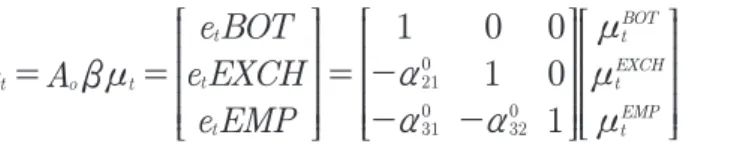
Again, Figure 3 depicts the trade balance trends for Nigeria from 1986 to 2021.
Figure 3: Nigeria’s Trade Balance from 1986 to 2021
Source: World Bank (2021)
It is evident from Figure 3 that the trade balance for Nigeria over a period of 35 years has shown net positive values representing the balance of trade surpluses, except for six years, that is, in 1998, 2016, 2017, 2018, 2019, and 2020, respectively. During the period under review, Nigeria’s balance of trade had the highest net surplus of US$84.54 billion in 2012, representing 18.56% of the GDP. The country’s trade balance had a net deficit of US$
25.01 billion in 2019, representing a 212.69% increase over the net deficit in 2018, while the net deficit of US$8.00 billion in 2018 represents a higher increase over the deficit in 2017.
Similarly, the trade balance deficit of US$ 0.02 billion in 2017 represents a 99.82% decline from the net deficit in 2016. Nigeria’s trade balance for 2016 was US$9.25 billion, representing -2.29% of the GDP. In 2021, Nigeria’s trade balance was also in a net deficit of US$ 6.49 billion, though better than the deficit of US$ 35.24 billion recorded in 2020, representing -7.25% of the GDP.
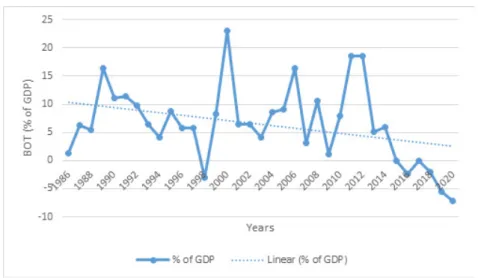
Nevertheless, the balance of trade for Nigeria from 1986 to 2021 is expressed as the
% of the GDP over these years, as shown in Figure 4.
Figure 4: Nigeria’s Trade Balance as % of GDP from 1986 to 2021
Source: World Bank (2021)
Figure 4 depicts Nigeria’s trade balance as a percentage of GDP from 1986 to 2021.
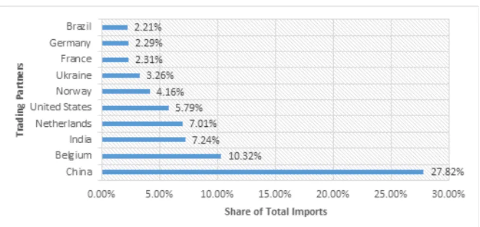
The trend shows a fluctuating pattern over this period. It exhibited both positive and negative movements. The figure shows a sustained negative trend from 2016 to 2021. When a linear trend was fitted, the trade balance showed a positive linear trend ranging from 10% in 1986 to 2% in 2021. Furthermore, Figures 5 and 6 depict Nigeria’s main trading partners in terms of exports and imports. Figure 5 presents Nigeria’s main import trading partners as of 2021.
Figure 5 shows the main import trading partners of Nigeria; the top import commodities in Nigeria include refined petroleum, cars, wheat, packaged medicaments, and telephones, which are mostly imported from China (27.82% of the share of total imports), Belgium (10.32%
of the share of total imports), India (7.24% of the share of total imports), the Netherlands (7.01% of the share of total imports), United States (5.79% of share of total imports), Norway (4.16% of the share of total imports), Ukraine (3.26% of share of total imports), France (2.31%
of share of total imports), Germany (2.29% of share of total imports) and Brazil (2.21% of share of total imports).
Figure 5: The Main Importing Trade Partners of Nigeria as of 2021
Source: World Bank (2022b)
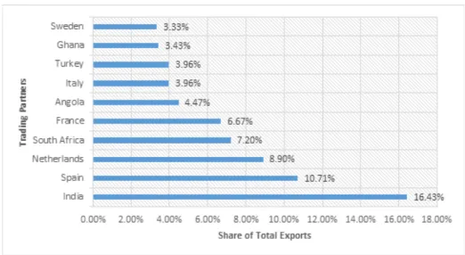
Finally, Figure 6 presents the top 10 export destinations of Nigeria as of 2021
Figure 6: Top 10 Exports Destinations for Nigeria as of 2021
Source: World Bank (2022c)
The export commodities of Nigeria include crude petroleum, petroleum gas, scrap vessels, and special purpose ships, which are mostly exported to India (16.43% of the share of total exports), Spain (10.71% of the share of total exports), the Netherlands (8.90% of the share of total exports), South Africa (7.20% of the share of total exports), France (6.67% of the share of total exports), Angola (4.47% of the share of total exports), Italy (3.96% of the share of total exports), Turkey (3.96% of the share of total exports), Ghana (3.43% of the share of total exports) and Sweden (3.33% of the share of total exports).
Preliminary Analysis
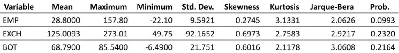
This section provides the preliminary analysis of the investigation, beginning with the descriptive statistics of the series used, and the unit root test results follow this. The descriptive statistics are presented in Table 1.
The table presents the descriptive statistics of the study’s variables. The table indicated 28.80 points as the mean value of EMP. It also showed 157.80 points as the maximum value of EMP in 2009. This period corresponds with the global financial crisis of 2009, which affected foreign exchange in the country. Its minimum value of -22.1 points coincided with 2008 when
the oil prices surged to an annual average of $99.67 per barrel, which enhanced foreign exchange inflows in the country. The normality test statistic has a value of 2.0626, which is not statistically significant, implying that the distribution of EMP is normal.
Table 1: Descriptive Statistics of the Variables
Variable Mean Maximum Minimum Std. Dev. Skewness Kurtosis Jarque-Bera Prob.
EMP 28.8000 157.80 -22.10 9.5921 0.2745 3.1331 2.0626 0.0993
EXCH 125.0093 273.01 49.75 92.1652 0.6973 2.7583 2.9217 0.2320 BOT 68.7900 85.5400 -6.4900 21.751 0.6016 2.1178 3.0608 0.2164
Also, the table further revealed 125.00 percent as the mean of the real effective exchange rate. It had a maximum value of 273.01 in 1998 and a minimum value of 49.75 in 1992. This minimum value of the exchange rate in 1992 may be ascribed to the performance of the monetary policy in 1992 that improved the overall economic performance of the economy at that time, while the surge in it in 1998 may be due to the wide differential between the official and black-market rates caused by the upsurge in foreign exchange demand in the economy. The normality test statistic has a value of 2.9217, which is statistically insignificant.
This suggests that the distribution of the real effective exchange rate is normal.
Again, Table 1 indicates the mean value of US$68.79 billion for the balance of trade, with a maximum value of US$ 85.54 billion in 2012 and a minimum net deficit of US$ 6.49 billion, coinciding with the year 2021. The surge in trade balance in 2012 may be ascribed to improvement in the merchandise trade, while the deficit in 2021 may be attributed to the COVID-19 pandemic that ravaged the global economy by truncating trading activities globally.
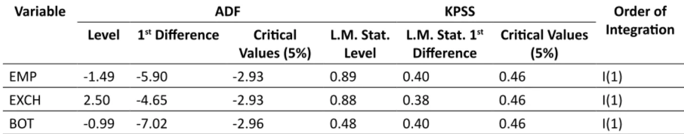
Furthermore, to avoid spurious outcomes in the regression estimates, unit root tests were carried out using the Augmented Dickey-Fuller (ADF) and the Kwiatkowsi-Phillips- Schmidt-Shin (KPSS) methods, and the results are presented in Table 2.
Table 2: Unit Root Tests Results
Variable ADF KPSS Order of
Integration Level 1st Difference Critical
Values (5%) L.M. Stat.
Level L.M. Stat. 1st
Difference Critical Values (5%)
EMP -1.49 -5.90 -2.93 0.89 0.40 0.46 I(1)
EXCH 2.50 -4.65 -2.93 0.88 0.38 0.46 I(1)
BOT -0.99 -7.02 -2.96 0.48 0.40 0.46 I(1)
The outcomes of both the ADF and KPSS tests revealed that the variables are stationary after the first Difference. This means accepting the alternate hypothesis that the variables are stationary. This suggests that the variables are resilient to shocks and can revert to their means in the event of any shock to the variables. This implies that any shock to the series will fizzle out over time. Again, the lag selection criteria were estimated to ascertain the appropriate lag order for the SVAR, and the results are presented in Table 3.
The estimated lag order selection criteria have revealed that the sequential modified L.R. test statistic, Final prediction error (FPE), Akaike information criterion (AIC), and Hannan- Quinn information criterion (H.Q.) have all shown that the optimal lag for the SVAR is lag 2.
However, lag 1 was used since the Schwarz information (S.C.) is preferred in lagged models. Its superiority over other alternative lag-length selection criteria stems from its ability to produce a more parsimonious number of lags than other criteria (Anne & Emily, 1988).
Table 3: Optimal Lag Selection Criteria
Lag LogL LR FPE AIC SC HQ
0 -849.7687 NA 9.81e+18 55.08185 55.26688 55.14217 1 -757.5808 154.6378 7.28e+16 50.16650 51.09166* 50.46808 2 -734.8898 32.20661* 5.01e+16* 49.73482* 51.40010 50.27766*
The Analysis of Long-Run Relation of Foreign Exchange Market Pressure, Exchange Rate, and Trade Balance
Following the outcome of the stationarity test and lag selection criteria, the Johansen co-integration test was conducted to ascertain the existence or otherwise of the long-run relationship among the variables, and the results are presented in Table 4.
Table 4: Rank Test (Trace)
Hypothesized Trace 0.05
No. of CE(s) Eigenvalue Statistic Critical Value Prob.**
r = 0* 0.632720 50.75017 47.85613 0.0232
r 1 0.417720 17.70126 29.79707 0.5882
r 2 0.047272 1.477154 15.49471 0.9991
r 3 0.000812 0.024367 3.841466 0.8759
The trace statistic shows one co-integrating equation among foreign exchange market pressure, exchange rate and balance of trade in Nigeria. This suggests rejecting the null hypothesis of no co-integration among the variables. Furthermore, the maximum eigenvalue statistic was computed, and the results are presented in Table 5.
Table 5: Rank Test (Maximum Eigenvalue)
Hypothesized Max-Eigen 0.05
No. of CE(s) Eigenvalue Statistic Critical Value Prob.**
r = 0 * 0.632720 30.04891 27.58434 0.0236
r 1 0.417720 16.22410 21.13162 0.2120
r 2 0.047272 1.452787 14.26460 0.9984
r 3 0.000812 0.024367 3.841466 0.8759
Also, the maximum Eigenvalue statistic has shown one co-integrating equation among foreign exchange market pressure, exchange rate, and balance of trade in Nigeria. This led to rejecting the null hypothesis of no co-integration among the variables. Therefore, the two statistics indicate the presence of co-integration among exchange market pressure, exchange rate, and balance of trade. The normalized co-integration equation was estimated to further ascertain the direction of this relationship among these variables. The estimates are presented in the following equation:
BOT = 24.82 + 1.94*EXCH + 1.28*EMP t 1.89 1.68 1.17
The above results have revealed a positive long-run relationship between the exchange rate and balance of trade in Nigeria, though statistically insignificant. This suggests that the pressure in the exchange market can potentially improve the balance of trade in Nigeria. Also,
the results showed that the pressure in the exchange market has a weak positive effect on the balance of trade in the long-run. This also indicates the potential for naira depreciation to improve the balance of trade in Nigeria. The exchange rate coefficients and pressure in exchange market pressure are greater than unity. The magnitudes of the coefficients align with the M-L condition that when the coefficient of elasticities is greater than unity, depreciation improves the economy’s trade balance with depreciating currency. However, the findings are at variance with the findings of Akpansung (2021), Usman and Bukar (2020), and Sanni et al. (2019), whose findings indicated that currency depreciation does not exert a positive impact on the trade balance in Nigeria; the findings though corroborated that of Odili (2014) whose finding revealed that currency depreciation has a positive but statistically insignificant long-run relationship with the balance of trade. The variation in the findings of this study compared to some of the previous studies may partly be explained by the choice of exchange rate variable. Some of these studies used nominal exchange rates, but this study used a real effective exchange rate that measures the value of Nigeria’s naira against a weighted average of currencies of many trading partners of Nigeria.
Short-Run Relationship among Foreign Exchange Market Pressure, Exchange Rate, and Trade Balance
Furthermore, to ascertain the short-run relationship between foreign exchange market pressure, exchange rate, and trade balance in Nigeria, the contemporaneous coefficients were estimated, as shown in Table 6.
Table 6: Results of the Contemporaneous Coefficients
BOT EXCH EMP
BOT 1 0 0
EXCH -1.633960* 1 0
EMP -3.778275* 9.927396* 1
*Denotes 5% level of significance
The results of the contemporaneous matrix have revealed that foreign exchange market pressure significantly exerts a positive effect on the exchange rate contemporaneously.
This means that if the pressure in the exchange market increases by 1%, the exchange rate in Nigeria will contemporaneously depreciate by 9.93%. This indicates that surges in the foreign exchange market pressure precipitate exchange rate depreciation in the country. This research outcome is in line with that of Kpoghul et al. (2022), who found that foreign exchange market pressure precipitated by global economic policy uncertainties, in turn, caused the exchange rate in Nigeria to depreciate.
Also, the results have shown that the exchange rate significantly negatively affects the balance of trade in Nigeria in the short-run. This suggests that if the exchange rate contemporaneously increases by 1%, it will cause the balance of trade to decrease by 1.63%
in the country. This research outcome is in line with that of Bahmani-Oskooe et al. (2018) and Mwito & Luvanda (2021), who found an inverse relationship between exchange rate depreciation and trade balance in the short-run, which marks the first phase of the J-Curve effect. Theoretically, both the M-L and the J-Curve theories posit that currency depreciation will alter the relative prices of domestic and foreign goods and the resultant effects on a depreciating economy’s trade balance. That is, the depreciation of a currency will make imports costly and exports cheaper, thereby reducing the current account of the depreciating country.
According to Doroodian & Roy (1999), the consumption of costly imported goods and the demand for low-price exported goods will subsist in the immediate period since consumers of expensive imported goods will be exploring cheaper substitutes, while the consumers of cheaper exported will adjust their absorption capacity to accommodate the supply of these goods.
Post-Estimation Tests of the Results
Before analyzing the shocks and the innovations among the variables, the diagnostic tests were estimated to ascertain that the estimates were free from econometric problems.
First, the VAR residual serial correlation ML test was conducted to check for autocorrelation in the SVAR model, as shown in Table 7.
Table 7: SVAR Residual Serial Correlation LM Tests
Lag LRE* stat Df Prob. Rao F-stat Df Prob.
1 20.14620 16 0.2137 1.328984 (16, 46.5) 0.2207
2 25.15846 16 0.0671 1.745026 (16, 46.5) 0.0709
Lag LRE* stat Df Prob. Rao F-stat Df Prob.
1 20.14620 16 0.2137 1.328984 (16, 46.5) 0.2207
2 37.25064 32 0.2401 1.210495 (32, 42.2) 0.2778
The SVAR residual serial correlation LM test results have shown that both the LM-stat at lag 1 and 2 have probability values greater than the 0.05 cut-off threshold. This, therefore, means the absence of serial correlation in the SVAR. That is, successive errors in the SVAR model are not highly correlated with each other. Second, the SVAR heteroskedasticity tests were conducted and presented in Table 8.
Table 8: VAR Residual Heteroskedasticity Tests
Joint test:
Chi-sq Df Prob.
186.7497 160 0.0727
Individual components:
Dependent R-squared F(16,14) Prob. Chi-sq(16) Prob.
res1*res1 0.925598 10.88537 0.0000 28.69352 0.0261
res2*res2 0.532809 0.997896 0.5062 16.51708 0.4175
res3*res3 0.597905 1.301100 0.3133 18.53504 0.2935
res4*res4 0.791842 3.328543 0.0145 24.54711 0.0782
res2*res1 0.854457 1.136961 0.0018 26.48816 0.0475
res3*res1 0.812775 3.798526 0.0080 25.19603 0.0664
res3*res2 0.666188 1.746235 0.1504 20.65182 0.1923
res4*res1 0.810385 3.739610 0.0086 25.12193 0.0677
res4*res2 0.792319 3.338183 0.0143 24.56187 0.0779
res4*res3 0.731077 2.378723 0.0552 22.66340 0.1230
The table shows the VAR Residual Heteroskedasticity Tests (Includes Cross Terms) with both the joint test and individual components. In each case, the Chi-square statistic values are not statistically significant, implying the acceptance of the null hypothesis that there is no presence of heteroskedasticity in the SVAR model.
Analysis of Shocks and Innovations of the Variables
First, the Impulse Response Functions (IRF) were analyzed. The IRF describes how each variable in the SVAR system responds to shocks from the system variables. Therefore, the impulse response functions were estimated and presented in the following figures. First, the impulse response of the balance of trade to the exchange rate was computed and presented in the following figure.
-1,200 -800 -400 0 400 800 1,200
1 2 3 4 5 6 7 8 9 10
Response of BOT to EXCH Innovation using Cholesky (d.f. adjusted) Factors
Figure 7: Impulse Response of Balance of Trade to Exchange Rate
From the impulse response graph, it is clear that in the first year, the shock in the exchange rate has caused the balance of trade to decline. The declining effect continued up to the fourth year; this marks the short-run effects. From the graph, the Marshall- Lerner condition is achieved in 4 years 6 months. This is predicated on the assumption that consumers have found domestic substitutes for imported expensive goods and services. Also, foreign consumers of trading partners may have switched from expensive imports to their own domestically produced goods and services. The Marshall-Lerner condition captures this linkage of price elasticities of demand for exports and imports. At this point, depreciation improves the trade balance (Onakoya et al. 2018). However, the graph did not exhibit a steep increasing trend over the forecast horizon. This suggests the potentiality of J-Curve in the dynamics of exchange rate and balance of trade in Nigeria. Again, the impact is permanent.
Moreover, the IRF of trade balance to foreign exchange market pressure was estimated and depicted in Figure 8.
Similarly, the impulse response graph of the trade balance response to foreign exchange market pressure exhibits the potentiality of the J-Curve effect. Initial shock in the pressure caused the trade balance to decline till the third period; after that, it began to increase but hovers in the negative part of the graph and became positive after the seventh year. Also, the effect appears to be permanent.
Finally, the Forecast Error Variance Decomposition (FEVD) was estimated. The FEVD offers information concerning the percentage of movements in a variable precipitated by its shocks and other shocks caused by other variables in the SVAR. Table 9 presents the FEVD of Foreign Exchange Market Pressure (EMP).
-1,000 -800 -600 -400 -200 0 200 400 600
1 2 3 4 5 6 7 8 9 10
using Cholesky (d.f. adjusted) Factors
Figure 8: Impulse Response of Balance of Trade to Foreign Exchange Market Pressure Table 9: Variance Decomposition of EMP
Period S.E. EMP EXCH BOT
1 83185.26 100.0000 0.000000 0.000000
2 95467.84 87.41959 7.232536 5.347876
3 97244.47 85.18857 9.654893 5.156542
4 98784.29 82.55372 9.357925 8.088360
5 100610.9 81.62492 9.030337 9.344745
6 101920.2 81.24839 9.272094 9.479515
7 102967.1 80.38690 9.793389 9.819715
8 104315.2 79.25318 10.14327 10.60355
9 106140.1 78.04259 10.48945 11.46797
10 108380.3 76.68037 11.02292 12.29671
The results showed that own shocks of foreign exchange market pressure are higher than other shocks from the beginning year to the last year, after which it reduced from 100%
in the initial year to 76.68% in the last year. It suggests that the exchange rate and the trade balance are the determinants of the pressure in the exchange market. This means that a unit change in exchange rate in the second period accounts for about 7.23% of the shock of EMP, and the effect increased significantly to 11.02% in the tenth period. Again, innovations in the trade balance account for 5.35% of the shock in EMP in the second period, and the effect improves significantly to 12.30% in the tenth period. The implication is that the exchange rate and the trade balance strongly predict EMP. Table 10 presents the FEVD of the Exchange Rate.
The results indicated that own exchange rate shocks are larger than other shocks from the initial year to the fifth year. It then declined from 38.81% in the fifth year to 28.70% in the tenth year. This means that the pressures in the exchange market and the balance of trade are the determinants of the exchange rate. Innovations in the balance of trade account for 6.06%
of the shock of the exchange rate in the initial year; the effect improved significantly to 32.01%
in the last year. Also, innovations in foreign exchange market pressure in the initial period account for about 2.59% of the exchange rate shock in the initial year; the effect increased