A generalized treatment of the order-disorder transformation in alloys and its effects on their magnetic properties

TRANSFORMATION IN ALLOYS

AND ITS EFFECT ON THEIR MAGNETIC PROPERTIES

Thesis by

Michael Baskes

In Partial Fulfillment of the Requirements

For the Degree of Doctor of Philosophy

California Institute of Technology Pasadena, California 91109

1970

(Submitted December 12, 1969)

I wish to express my sincere gratitude to Professor F. S.

Buffington who suggested the problems treated in this dissertation and offered valuable guidance in this research.

I would like to acknowledge the financial support of the National Science Foundation and the John and Fannie Hertz Foundation.

I also would like to thank Mrs. Vivian Davies for her help in typing the thesis.

Abstract

A theory of the order-disorder transformation is developed in complete generality. The general theory is used to calculate long range order parameters, short range order parameters, energy, and phase diagrams for a face centered cubic binary alloy. The theoretical results are compared to the experimental determination of the copper- gold system, Values for the two adjustable parameters are obtained.

An explanation for the behavior of magnetic alloys is developed, Curie temperatures and magnetic moments of the first transition series elements and their alloys in both the ordered and disordered states are predicted. Experimental agreement is excellent in most cases. It is predicted that the state of order can effect the magnetic properties of an alloy to a considerable extent in alloys such as Ni₃ Mn. The values of the adjustable parameter used to fix the level of the Curie temperature, and the adjustable parameter that expresses the effect of ordering on the Curie temperature are obtained.

TABLE OF CONTENTS

PAGE

I. Introduction 1

ll. Calculation of the Free Energy of an Alloy 5

A. Energy 5

B. Entropy 19

C. Free Energy Minimization 21

III. Application of the Order-Disorder Theory 24

IV. Magnetism in Alloys 41

A. Magnetic Properties of Disordered Alloys 51 B. Magnetic Properties of Ordered Alloys 67

1. Saturation moment 67

2. Curie Temperature 69

V. Conclusion 94

VI. References 97

Appendix I Values of N(H, i, I, k, J, j)/N~ for various lattice

structures and sublattices. 100

Appendix II Appendix III Appendix IV

Energy of a binary alloy on two sublattices. 104 Entropy of a binary alloy on two sublattices. 109 Minimization on the free energy of short range

order. 111

LIST OF TABLES

TABLE PAGE

I Values of w for various lattice structures and

II

III

IV

v

superlattices

Order parameters for a f,c .c. AB₃ stoichiometric alloy for p = 0

Values of m, J, u, g, B, n_{0 ,} T , and 0₀ for the first series transition elemen<f:s

Number of electrons element contributes to a nickel alloy

Number of electrons element contributes to cobalt alloys

VI - Number of electrons element contributes to iron alloys

15

26 49

52

59 66

FIGURE 1 2

3

4

5

6

7

8

9 10

11

12

13

14

LIST OF FIGURES

PAGE

The Slater-Pauling curve 3

Relationships between distances and sites used to

define N(H,i,I,k,J,j). 6

Relationships between atoms and sites used to

define p. (j3I

I

aH). 7

l

Long range (S) and short range (er. ,q/ q L) order

coefficients for the f.c.c. AB₃ ¹stoicniometric alloy

q = qAB = qBB 29

Long range (S) and short range (er. ,q/q ) order coefficients for the f.c .c. AB₃ ¹

stoic~iometric

alloy q = qAB = qBB 30

Long range (S) and short range (er_{1 )} order coefficients for f.c.c. AB alloys of various compositions 31 Energy of the f.c.c. AB₃ stoichiometric alloy for

various values of p 32

Energy of the f.c.c. AB₃ alloy for various

compositions 33

Energy of the f.c .c. AB alloy for various compositions 34 Partial phase diagram for p = 0 with no lattice

parameter variation 35

Partial phase diagram for p= .025 with no lattice

parameter variation 36

Partial phase diagram for p = -.025 with no lattice

parameter variation 3 7

Partial phase diagram for p = 0 including lattice

parameter variation 3 8

Partial phase diagram for p= -.025 including lattice

parameter variation 39

15 Experimental phase diagram of the copper-gold.system 40

16

Comparison of the values of BB commonly used and

the values used in this treatfnent 47

List of Figures (Cont¹d.)

FIGURE PAGE

1 7 Saturation moments and Curie temperatures of

nickel alloys 7 3

18 Saturation moments and Curie temperatures for the

nickel-cobalt alloys 74

19 Curie temperature of iron-nickel alloys under various

assumptions specified in the text 75

20 Saturation moments in iron-nickel alloys 76

21 Curie temperature of iron-nickel alloys 77

22 Saturation moments of nickel-manganese alloys under various assumptions specified in the text 7 8 23 Saturation moments of disordered nickel-manganese

alloys 79

24 Curie temperature of disordered nickel-manganese

alloys 80

25 Saturation moments and Curie temperatures for the

iron-cobalt alloys 81

26 Saturation moments and Curie temperatures of

cobalt alloys 82

27 Saturation moment and Curie temperature of iron

alloys 83

2 8 Saturation moments and Curie temperatures for the

iron-chromium alloys 84

29 Saturation moments and Curie temperatures of

30

31

32

iron-vanadium alloys

Theoretical values of the saturation moments of

.

nickel-manganese alloys for various degrees of long range order, S, and short range order, qAA1' qAB1' qBB1' q1

=

qAA1 = qAB1 = qBB1 Saturation magnetization of nickel manganese alloys

quenched from various temperatures, T Curie temperatures of nickel alloys with various

degrees of long range order, S

85

86

87

88

FIGURE 33

34

35

36

37

List of Figures (Cont'd.)

Curie temperatures of nickel alloys with various degrees of long range order, S

Curie temperatures of fully ordered nickel alloys for various values of the magnetic interaction parameter, A.₁

Curie temperatures of nickel manganese alloys with various degrees of long range order, S Curie temperatures of nickel manganese alloys with

various degrees of long range order, S Curie temperatures of fully ordered nickel

manganese alloys for various values of the magnetic interaction parameter, A.₁

PAGE

89

90

91

92

93

Introduction

It was first proposed by Tammann¹ that the atoms in an alloy may arrange themselves in an ordered structure. The first use of x-rays to show the presence of an ordered structure was made by Johansson and Linde² • Nix et al~ used neutron scattering to show the presence of order in alloys whose components had almost identical x-ray scattering factors. It is also possible to use electron diffraction⁴ to determine the presence of order in alloys.

The experimental evidence implies the existence of an ordered structure in which like atoms tend to surround themselves with as many unlike atoms as possible. Consideration of the free energy leads to the prediction that an alloy ordered at low temperatures will disorder at high temperatures where the temperature times entropy term becomes more important. Experimental evidence ⁵ ,& also implies that there are two kinds of ordering, long range order and short range order. If long

range order exists each type of atom migrates to a designated atomic site forming a superlattice.

There were many early theoretical attempts ^{7 , 8 ,9, 10} to explain the order-disorder transformation in alloys. Bragg and Williams ¹¹ introduced the most famous of these theories. Their treatment con- sidered only long range order, the AB type of superlattice, binary alloys of stoichiometric composition, and ignored atomic interactions other than those with first nearest neighbors. Their method was refined and extended by Bethe ¹², Peierls 13 , Chang 14 , Easthope ¹⁵ and others to include the short range order of first nearest neighbors, the

AB ₃ type of superlattice, and non- stoichiometric compositions. The extension to non-stoichiometric compositions, however, was incorrect as it did not predict a maximum critical temperature of long range order around the AB₃ stoichiometric composition contrary to experi- mental evidence.

Cowley ¹⁶ and Fournet ¹⁷ considered interactions with other than first nearest neighbor by assuming a small but arbitrary contribution from the second and third nearest neighbors. The contribution was

determined by those values that fit the experimental data best. Cowley¹s¹⁶ theory of short range order is quite good. In extending it to long range order, however, he erroneously considers only those atoms on a simple cubic lattice in taking the limit of the short range order parameters. He also errs in assuming that the superlattice sites are always available in the same ratio as the compositions of the atoms. This assumption leads to an incorrect dependence on composition.

The major deficiencies of the above theories are 1) insufficient generality in treating all crystal structures and superlattices; 2) im- proper treatment at the variations with composition; 3) incomplete treatment of the interaction of neighbors other than the first nearest;

4) inability to treat more than two components; and 5) inability to treat the combination and interaction of long and short range order.

Ordering in alloys can have rather dramatic effects on their magnetic properties. As one example, the ordered stoichiometric alloy Ni₃ Mn has a Curie temperature that is 600° higher than the disordered alloy. Grabbe¹⁸ has shown that ordering increases the saturation

magnetization of iron-nickel alloys with the largest increase near Ni₃ Fe.

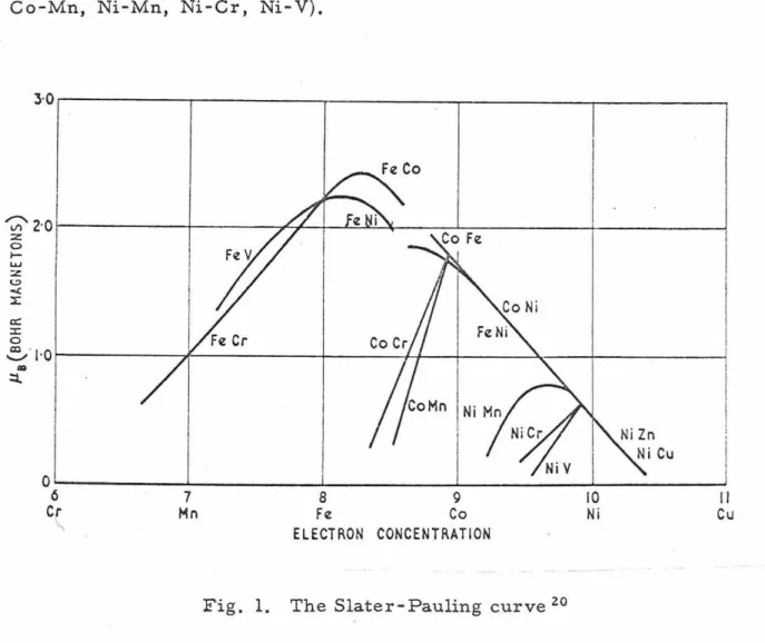
The variation in the saturation magnetization in disordered alloys is usually explained by considering the electron concentration.

The Slater-Pauling curve l9 (Fig. 1 ) shows that this relationship is usually valid, although there are some prominent exceptions (Co-Cr, Co-Mn, Ni-Mn, Ni-Cr, Ni-V).

~2·0r---j'---yc....r---J-~-"-'--+---l---l---l _::z

0 1-..,

:z

C>

~

:l:

a:

:I:

0

~

...

· 1·0 r - - - -- - --7'1' - - - -- - ---+- - --+-l'----!- - ---'"--- --+- -- - - ---!

~

o---~~~~~-'--~~~~~-...1~~~~~~....1...~~~~~-...1~~~~~~

6 Cr \

Mn 7 Fe ⁸ Co ⁹

ELECTRON CONCENTRATION

Fig. 1. The Slater-Pauling curve ²⁰

10 Ni

Goldman and Smoluchowski ²¹ have considered the saturation magnetization to be determined by the local electron concentration rather than the average electron concentration. Smolucho...vski ²² applied this idea to iron-cobalt alloys with good success. The appli- cation to other alloy systems has not been fruitful.

II Cu

Sato ²³ and Muto et al.²⁴ have made theoretical studies on the effect of order on magnetic properties without much success in develop- ing a working theory. Bell, Lavis, and Fairburn²⁵ have made a theo-

retical study on the equilibrium behavior of ordered magnetic alloys.

Their results are of a very qualitative nature and virtually impossible to compare with experiment without making simplifying assumptions that render the theory practically useless.

There has been little success in obtaining a comprehensive theory of magnetic behavior of alloys in either the disordered or ordered states.

The objectives of this study are 1) to derive a theory of the order-disorder transformation in sufficient generality so that it may be applied to any crystal structure or superlattice, multicomponent systems, and nonstoichiometric compositions; 2) to examine the behavior and

interaction of long and short range order; 3) to determine the effect of the interaction of neighbors other than first nearest; and 4) to explain the magnetic behavior of alloys and how it is influenced by ordering.

'-.

Calculation of the Free Energy of an Alloy

Energy

Consider a space lattice of N sites. Di vi de this lattice into sublattices of types designated by A, B, C, Let H,I, or J dummy indices each of which may be equal to A, B, C, Define n H(n

1, n J) as the fraction of sites contained in the Hth(Ith, Jth) sub- lattice. Since all sites are included in one or another sublattice:

be

~

^{nH = 1,}

~

^{n I = 1,}

~

^{n J = 1 (1)}

H I J

Define NIH i as the number of I sites that are

a

distance r i from an H site, where i = 1, 2, 3, . . . The number of I sites a distance

l

r i from all H sites equals n HNNIH" Similarly the number of H sites a distance r.

1

from all I sites equals n l

1NNHI. Since the number of I-H pairs at distance r . must equal the number of H-I

.]:

pairs at distance ri":

( 2)

For example, a body centered cubic structure may be divided into two interpenetrating simple cubic sublattices where n A =

i,

l l l l 1 z z

nB=z, NAA=O, NBB=O, NAB=8, NBA=B, NAA=6, NBB=6,

z z

NAB = 0, NBA = 0, etc.

Consider an H site. (Fig. 2) Look at all I sites at a distance

r. l from this H site.

6

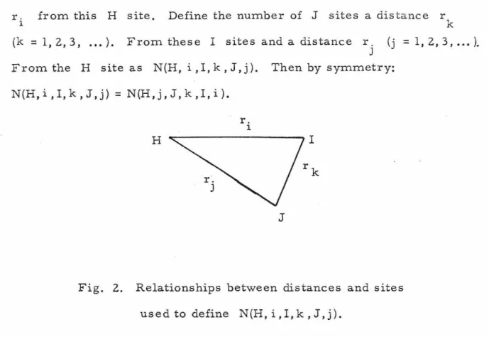
Define the number of J sites a distance r k (k = 1,2,3, ..• ). From these I sites and a distance r.

J ^(j = 1, 2, 3, ... ).

From the H site as N(H, i, I, k, J, j ). Then by symmetry:

N ( H, i , I, k , J , j ) = N (H , j , J, k , I , i ) .

H

r. l

J

Fig. 2. Relationships between distances and sites used to define N(H,i,I,k,J,j).

The values of N(H,i ,I,k, J,j) for various lattice structure and super- lattices are given in Appendix I.

An atom of types designated by a, b, c, ... , is located at each site of the space lattice. Vacant sites may be considered by assuming one type of atom to be vacancies. Let

a, f3,

^{or y} be dummy indices each of which may be equal to a, b, c, ... . Define m (mR, m ) as

a ,....

Y

the fraction of the

a

th (/3th, yth) type of atom. Clearly:

~ mf3

= 1,

f3

~

^m _y

=

^1.

y

(3)

Let the total number of

a

atoms on the H sites be given by

where Xa (H) is the probability of finding an a atom on an H site.

Since each site is occupied

for H=A, B, C, ... ^{( 4)}

Since the composition of each component is fixed

for

a

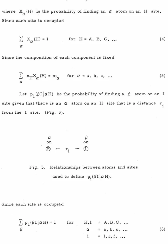
= a, b, c, ... (5)

Let p. ({31

I a

H) be the probability of finding a ,B atom on an I

l

site given that there is an

a

atom on an H site that is a distance r.

l

from the I site. (Fig. 3).

a

on

®

on

f3

r_l . -

CD

Fig. 3. Relationships between atoms and sites used to define · p. (,BI _l

1 - a

^H).

Since each site is occupied

I

^{Pi (,81 iaH) = 1 for H,I = A,B,C,}

{3

a

= ^{a, b, c,}

i = ^{1, 2, 3,}

...

( 6)

8

The total energy, E, may be calculated by considering each atom successively as the origin and then adding the energies of all atom pairs. The energy so calculated must be divided by 2N as each inter- action has been counted 2N times. If E

f3

y(rk) is the interaction energy between a [3 and y atom separated by a distance rk;

E

=

₂^1N

L.

^{nHNXa (H)} N(H, i,I,k, J,j) 1jka

f3

yHIJ

EjQ (rk)p. (f3IiaH) p.(yJ!aH)

fJ y ^l J

(7)

The total energy may also be calculated by the classical method of considering successively one site of each sublattice as the origin and adding the energies of interaction of all atoms with the atom at the origin. In this way

E =

± L.

kf3

yIJ

The factor of

±

is due to counting each interaction twice.

The energy may be separated into two parts, ELRO' the contribution from long range order only, and ESRO the remainder.

Let

p. (/3IlaH)

=

X{3(I) (l+q. (,BiiaH))

l l

and similarly

p.(yJiaH) = X (J) (l+q. (yJiaH))

J y J

(7a)

(Sa)

(Sb)

9

The set of qi and ~ so defined are a quantitative measure of the short range order. They are equal to zero in the absence of short range order. The set of X's are a quantative measure of the long range order.

Equations (4), (6), and (8) yield:

L x

13

^{(I) qi ({3I I a H) = 0}

f3

and

L ^x

(J)q. (yJlaH) = 0 y J

Ci.

(9a)

(9b)

Since the number of

a

-{3 atom pairs at a distance r. is equal

l

to the number of

f3

-a atom pairs at a distance r. :

l

L

^nHXa (H)pi ({3 I I ^a

H)N~H

⁼

L

ⁿ₁Xf3 (I)pi ^(a HI

f3

I

)N~

HI IH

i i

From equation (2) · nHNIH

=

^~NHI which with equation (8a) yields:

For

L nHN~HXa(H)Xf3(I)[qi(,8Ila.H)

^{- qi(a.Hlf3I)J}

⁼

^O

HI

~NIH l Xa(H) X\3 (I) =I= 0 q. (/3IlaH) = q. (aHlf3I)

l l

Similarly

q .(yJlaH) =q.(aHJyJ)

J J

(lOa)

(lOb)

Equations (lOa, b) are also valid for the trivial case

~NIH 1 Xa (H) Xf3 (I)

=

0. Using equations (Sa, b) in equation (7):

E -- .^.!. z

2::

nHXa (H) N(H, i 'I' k, J' j) E

f3

'Y(rk)

xf3

(I) x'Y (J) ijka

f3

'Y HI J

[l+q.(f3IiaH) + q.(-yJlaH) +q. (f3IiaH)q.(-yJiaH)J

1 J 1 J

The summation over

a

of the second and third terms in brackets above may be written:

=

=

2::

^Xa(H) [qi({3I)aH) + qj(-yJlaH)J

a

2::

^Xa(H) [qi(aHif3I)

+

qj(aHhJl]

a

l, ^x

13 (i)qi(,BIJaH) + l:xa(J) qj(-yJJaH) =

o

f3

'Y

where equations (9a, b) and (~Oa, b) have been used and the dummy indices have been changed,

Equation (7) may now be written:

E

=

^ELRO

⁺

^ESRO

where

ELRO =

i 2::

^nH

xa

(H) N(H, i, I, k, J' j) E/3 'Y(rk)Xf3 (I)X)J) ijka

f3

'Y HIJ

(11)

ESRO = i

~

nHXa (H) N(H, i, I, k, J ,j) Ef3 y(rk)X{3 (I) Xy(J) ijka f3 y HIJ

q. ({3 I

I ^a

^{H) q. ( yJ}

I ^a

^H)

l J

Similarly we may separate equation (7a) into two parts.

ELRO = iN

~ ~N;I

^{X{3 (I) Xy(J) Ef3 y(rk)}

k{3 yIJ

ESRO = iN

~

_.

nIN~I

^{x{3 (I)}

x

_y ^{(J) qk ( y J I {3 I) E{3} _y ^(rk)

k{3 y IJ

(12)

(lla)

(12a)

Equation (11) may be simplified considerably. Consideration of the summations over

a ,

j, i, and H yields: ¹

~

^nH

~~

N(H,i,I,k,J,j)

~ ^xa

^(H)

H i j

a

= _~

^nH

~ ~·

^{N(H, i,I, k, J, j)}

H l J

~ ~

^{i k}

=

nH NIH NJI

H i

L:

^{k k}

=

^{nH nI NNJI}

=

^{nI N NJI}

H

l

The summation over j may be performed by first considering one I site a distance r. from the H site. The number of J sites a

l

distance rk from this I site and any ( ; ) distance from the H site is simply

N~

^I" Now simply multiply .by the number of I sites a distance ri from the H site, i.e. NIH' l

Equation (11) m:ay now be written

kf3yIJ

~ ^NJI k

12

which is identical to equation (lla) which was calculated by the classic al

method.

Next, consider the summation over k in equation (lla).

Ordinarily approximations have been introduced at this stage such as the Bragg-Williams approximation of considering only the contribution from the first nearest neighbors, i.e. k = 1. Others have attempted to include the effect of second nearest neighbors by assuming a small, arbitrary contribution from them. The complexity introduced by con- side ring other neighbors was usually assumed to be too much to handle.

This investigation was undertaken, in part, to determine if the above approximations were indeed necessary. The development that follows leads to the conclusion that in many cases of interest the symmetry of the lattice is sufficient to insure that none of these limiting assumptions need be made.

Let

N~

^be the number of. sites that are a distance rk from an I site.

N~

⁼

~

J

k k

I

^k

Let cJI = NJI NI which implies

~ c~I

= 1. For each rk there is a set of

c~I.

Some of these sets ^J of c JI ^k may be identical for different values of k . . Each such group of sets shall be designated

by k (n=l,2, ... ).

n

k n

The characteristic set of c JI shall be designated by w n JI' From above

(13)

The summation over k in equation (lla) now becomes:

n

If the crystal symmetry is sufficient to insure that the number of kth neighbors to a site is independent of the site, i.e. NI ^k = N then ^k the summation over k in equation (lla) becomes

l: w~I E~y

⁽¹⁴⁾

n k

where

E~y = l:

N n E.BY(rn) =

E~ f3

equation (lla) becomes: k n

E l.N

LRO

=

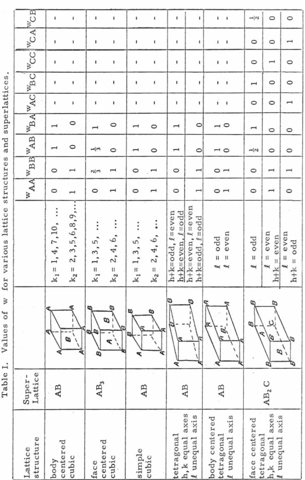
^{2 (15)}

The value of replacing the summation over k by the summation over n may be seen by considering a brief example. In the face-

centered cubic AB structure there are only two sets of wn JI' For

k1 =1,3, 5, ... w1_B = wBA = ~. ^{W I} AA ^-- ^wBB ^l =~

k₂

=

2, 4, 6, ... ^Wz - wZ - 0

AB - BA - '

WAA ⁼

^{w2B B}

⁼

^{l •}

A similar result is found for the simple cubic AB structure, tetrago- nal AB structure, body centered tetragonal structure, face centered cubic AB₃ structure and the body centered cubic AB structure

(Table 1). In the above cases the summation over n in equation (15) is therefore over only two values of n. For the face centered tetrago- nal AB₂ C structure, the summation is over three values of n (Table I).

It is interesting to compare the above example with the approxi- mation of k = 1, 2 (second neighbor) of equation (lla). For equation (lla) the summation over k becomes:

while in equation (15) the summation over n becomes:

The mathematical complexity of the exact equation (14) is no more complicated than using the second neighbor approximation, yet equation (15) considers all atomic interactions.

It must be remembered that Ef3¹ and E²

f3

are the weighted

' y y

sums of all atomic interactions, while Ef3y(r_{1 ),} Ef3y(r_{2 ),} Ef3y(r_{3 ), ...}

represent the interactions at first, second, third, ... neighbor distances.

Table I. Values of w for various lattice structures and superlattices. Lattice Super-I structure Lattice WA.A WBE WAB WB.A WAC WBC A A body AB

/l/

k1 = 1, 4, 7, 10, 0 0 1 1 centered A '

...

-

-

cubic

s: I/A

kz = 2, 3,5,6,8,9, ... ,,.-1 1 0 0 A ,,,, -

-

A J::I face e/"' ii k1 = 1, 3 I 5 I • •• 0 2. l centered AB3 I 3 3 1

- -

cubic A I 8 8 kz = 2, 4, 6, ... ,. , --1 1 0 0 ,.

- -

, .., simple AB

ArjJ

k1=1,3,5,

...

0 0 1 1

- -

cubic .... --· -8 k2 = 2, 4, 6, •.. 1 1 0 0

- -

A tetragonal A~--Jf-·fJ h+k odd, P. even h, k equal axes AB

..,

h+k=even. P. =odd 0 0 1 1

- -

, I P. unequal axis

- --

^·-

... ....!_ --8 h+k even, P. even ~ ,. h+k odd . .£-odd 1 1 0 0

- -

body centered

· ~~11

tetragonal AB A . i = odd 0 0 1 1 VJ B'

- -

i. unequal axis

,,.--~;ti

i = even 1 1 0 0

- -

,., face centered B Q i = odd 0 0 1 tetragonal

8 ~ 8

2 1 0 1 h,k equal axes AB2C 1 even 1 unequal axis h+k = even 1 1 0 0 0 0 B ,,.,

--

J_ ,_ ,, even b '8 h+k = odd 0 1 0 0 1 0

wee

WCA

- - -

- --

- -

-

-

--

- - - - - -

-

-

0 0 1 0 0 1

l\vCE

- - - - - - - - - -

l 2 0 0

16

Equation (12a) may be simplified in a manner similar to that used in the simplification of equation (lla) above. Let r be the

n

smallest of rk . The summation over k in equation (12a) may be n

written:

k k

\ ' \ ' n n

I

= Li Li cJI NI qk (yJ {3I)E{3 (rk)

k ⁿ Y n

n n

+ I: w~I

n

Since I E,By(rk) I decreases rapidly with increasing rk' it is safe to assume IE{3 (3k) I<< IE/3 (r )

I

k 1= n and to ignore the second

y n y n n

summation. This approximation is better than the usual second neighbor approximation for three reasons:

1) This approximation is made in the short range order energy term, while the usual approximation is made in both the long and short range order energy terms. Usually the energy of short range order is much less than that of long range order thus the above error is correspondingly less.

2) In the case of a large amount of short range order q - q thereby

k n

n reducing the error.

3) For some structures the energy assumption is lessened, In the face-centered cubic case the third neighbor interactions are

consider the order-disorder transformation in binary alloy systems.

Specific consideration will be given to lattice structures that may be decomposed into two sublattices, such as the face-centered cubic and body-centered cubic systems. For the above special case equations (15), (12) and (17) become (Appendix II).

ESRO

=

²

Ii

iIJ

(19)

+

^\'.L! ^' nHN(H,i,I,k, J,j) x:(H) ^{X (H)}

Xa (I)Xa(J)q~Hqk

^{. . ~E. Nk ab(rk)}

ijkHIJ

\ ' l

where L! is over i,j,k

>

⁰

E = energy of an ¹¹ a¹¹ aa

Ebb= energy of a llbll E ab - energy of a 1lb1l or energy of an ¹¹a 11

atom in pure atom in pure atom in pure atom in pure

~Eab = (Eaa

+

Ebb - 2Eab) Hall llb'' 11a11

"b"

~Eab(ri)

^{= Vi(Eaa(ri)}

⁺

Ebb(ri) - 2Eab(ri))Ni

~E~b

⁼

L ^~Eab

^{(rk )}

n n

The above derivation is givenk in Appendix II.

(20)

( 21)

19

Entropy

Consider the entropy contribution from the long and short range order of all atoms that are separated by a distance r ..

1.

The number of I sites at a distance r. from an a atom on

1.

an H site is

sites is

where

The number of {3 atoms on these I sites is

The number of ways of arranging these

f3

atoms on these I

( n ) _ n!

k - n!(n-k)! •

The number of ways of arranging all (3 atoms at a distance r.

1.

from any atom on any site is

n

a

HI

The number of ways of arranging the

f3

atoms after the y atoms have been arranged on I sites is

TT

a

HI

The number of ways of arranging all atoms at a distance r .

l

from any site is:

-II

ia

f3

HI

. {3-1

N~H

Xa(H) nHN(l -

~

pi (yI

I

^aH))

. y=l

W= _{( 22)}

The entropy, S, is obtained from

S = K ln W

where K is Boltzmann¹ s constant.

In the special case of a binary alloy on two sublattices, the entropy takes the form (Appendix III):

(23)

where

G(x) = x i nx

+

(1-x) in(l-x)

The derivation of (23) is given in Appendix III.

i i

*

It is useful to obtain the form of the entropy in which qIJ = qIJ

for all i .

The value of i

·*

is the lowest value of i which yields the correct entropy in the limit of perfect short range order. For b. c. c.

*

^''<

i =l, for £. c. c. i"= 2. In this case:

S = -NK

~

^{ninJ{ Xa (J) c} (xa (I)(l-qiJ

*

)) IJ

Free Energy Minimization

First consider the free energy dependence on short range order.

Using the general formula

F = E - TS

where F is the free energy, E, the energy, T the absolute tem- perature, and S, the entropy, minimize the free energy with respect to the short range order parameters. E is obtained from equation (20) and S from equation {23). The resulting set of equations is given below for each I, J, i :

. X (I) X (J) .

2~E

^{b(r.) (1}

⁺ q~J)

⁽¹

⁺

x: (I) x: (J)

q~J)

a i

+

£ n

---=----=---

Ni K T X (I) . X ( J) . (1- x:(r)

q~J)

^{(1- x:(J)}

q~J)

+ ~1

jkH

[

N(J,i,I,k,H,j)

q~

N(I,i,J,k,H,j)

Xa(H) i X (J)+ i

NIJ b NJI

=

0

The derivation of equation (25) is given in Appendix IV.

(25)

The set of equations (25) may be solved by the following iteritive procedure: Let

[

N(J,i,I ,k,H ,j) qJH i X ( H) . _..:.;=-=-

a N1 Xb(J)

IJ

N (I, i, J, k, H, j )

X (I) X

=

^a

Xb (I) '

x

^{(J) i·}

y

=

^{a Q}

Xb(J) ' = qIJ

Equation ( 25) may be written:

(l+Q)(l+ XYQ)

£nD + £n (1-XQ)(l-YQ)

=

⁰

(l+XY) D + x + y - /[(l+XY)D+ x+ Y]

2

-4XY(D-lt Solving for Q: Q=

2XY(l-D)

l l

A set of qIJ is assumed (q

11

=

0 is a good starting point). For a

given X, Y, and

.6E b(r.) a i

D is calculated. Next, Q is

calculated and the old value of qIJ is i replaced by the new one. The

procedure is repeated until the calculated Q is as near to the trial Q as desired.

It is now possible to calculate a set of qIJ for any i given long

range order and temperature, To minimize the free energy with respect to the long range order parameter, use the set of qIJ i determined above

along with the energy of equations (19) and (21) and the entropy of

equation (24). Values of the long range order parameter are assumed and the free energy is calculated until a minimum is obtained.

Application of the Order -Disorder Theory

The following assumptions have been made to facilitate the calculations:

(1) Short range order parameters for shells greater than a distance of 10th nearest neighbors are set equal to zero.

(2) To avoid the choice of numerous arbitrary constants, the following energy values are assumed in the calculation of short range order parameters:

k > 2 '

i.e. the 6.E values at first and second neighbor positions are given by the 6.E values for the odd and even shells respectively. Assumption

(1) has very little effect on the results obtained below since the short range order parameters for shells greater than 10th nearest neighbors are small (Table II) . In addition, the effects of the atoms in these distant shells frequently cancel. Assumption (2) has little effect on the results obtained below except perhaps for a small effect on the values of the short range order parameters in the shells greater than 2nd nearest neighbors. For example, if 6.Eab(r_{3 )} =f. 0 there is a change in the

short range order parameters of the third shell. For

i

^{L::.Eab (r}_{3 )} ^J < <

J6.Eab(r_{1 )}

I ,

however, the effect is not great. It therefore seems

reasonable as a first approximation to ignore 6.Eab (rk) for k

>

2.

Use of the dimensionless quantity K.T / 6.E~b permits the

1

determination of ~Eab by comparison with the experimental critical

2

temperature. The remaining energy ~Eab will be used in the form

2 1

~Eab/ ~Eab

=

p. The behavior of an alloy system will be examined as a function of p. A long range order parameter, S, may be defined as:

s =

^{X a (A)-m a}

nB

This parameter reduces to the Bragg-Williams S for stoichiometric compositions. A short range order parameter, CT i, for each shell may be defined as:

where N ^l (S, q) aa

CT. =

l

i i

N (S,q) - N (S,O)

aa aa

N i (O,qL)

aa ^Ni aa ^{(0, 0)}

is the number of a-a atom pairs at distance r . with

l

l i

long range order S and short range order q given by qAA, qAB , qBB and qL is l the maximum short range order possible. The param- eter CT. is equal to zero for no short range order and equal to one for

l

maximum short range order.

For structures such as face centered cubic, with m > . 25, the a

fully ordered structure has some a-a first neighbor pair?. The limit- ing values of q determined above yield no a-a first neighbor pairs, i.e. q - -1. ^It is therefore necessary to multiply the q values

i mb

determined above by ₃ m for ma> .25. This procedure gives the a

proper qL values.

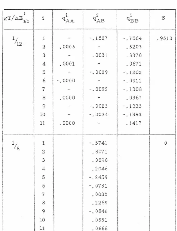
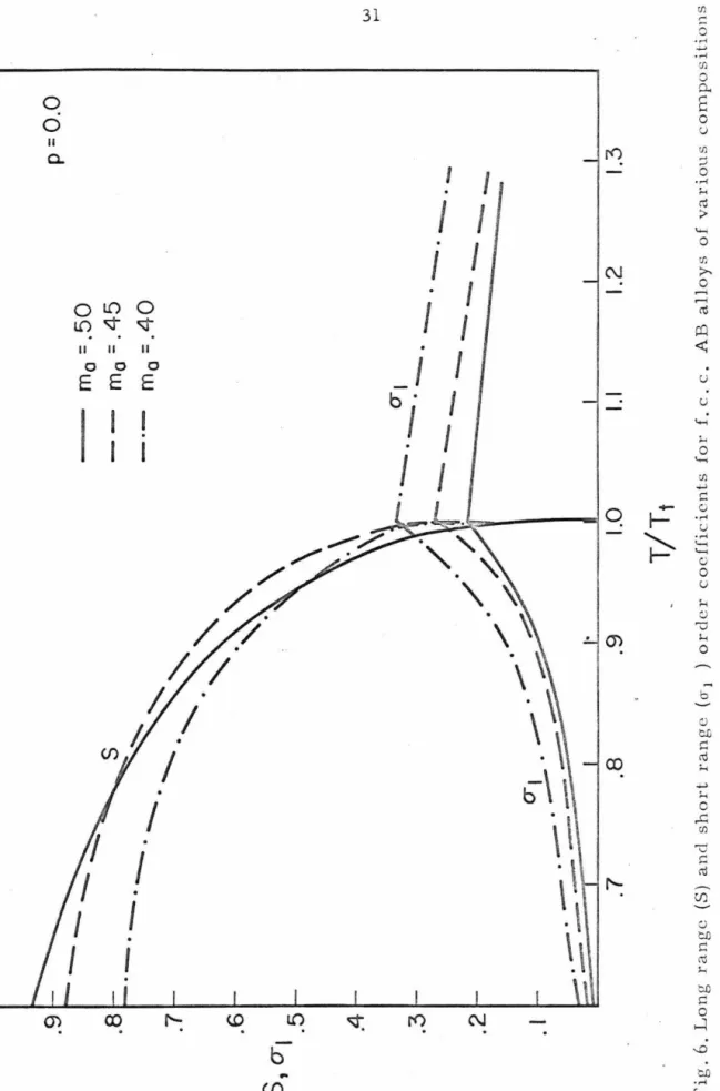
Table II shows typical order parameters for an AB₃ stoichiom- etric alloy. Figures 4-6 show S, CTi' and q/qL as a function of

1

l

KT/ 6.Eab

1 112

I I

I

_I

1/ 8

i

1 2 3 4 5 6 7 8 9 10 11

1 2 3 4 5 6 7 8 9 10 11

TABLE II

I

i i

qAA qAB

- I ^I

I -.1527 . 0006

-

-

. 0031 . 0001 -

- -.0029

-.0000 -

- I

^{-. 0022}

.0000 -

-

!

-. 0023

- -

. 0024

. 0000

-.5741 . 8071 . 0898 .2046 -. 2459 -.0731 . 0032 . 2269 -,0846 . 0331 .0666

I

I l

t

i I

I

!

I

I _t'

I

I

I

I I

i qBB

- . 7 564 .5203 . 337 0 . 0671 -.1202 -. 0911 -.1308

0 0367 -.1333

-

.1353 . 1417

s

I

^{. 9513}

i

i

I

I

I ! l

J

I

0

Order parameters for a f. c. c. AB₃ stoichiometric alloy for p

=

^0.

I I

I

I I

T/Tt and p for various compositions and lattice structures, where T t is the highest temperature at which long range order exists.

Figures 7-9 show the energy as a function of T/Tt and p for various compositions and lattice structures. Figures 10, 11, and 12 show partial phase diagrams for different values of p. The two phase regions were determined by the common tangent method.

In the phase diagrams the disordered regions represent alloys with no long range order, but with a varying degree of short range order. The ~ B, AB, and AB₃ regions represent alloys with varying amounts of long range order based on the respective superlattice plus a varying amount of short range order.

2

For p = 0, i. e, t!.Eab = 0, three maxima (2.5 % , 50 % , 75 % ) are observed. For the case of no lattice parameter variation, two eutectoids occur at a temperature 67 .5

%

of the critical temperature for the AB stoichiometric alloy (Fig. 10). For p = .025 the three maxima are again observed, however no eutectoids occur (Fig. ll).

For p

=

-.025 one maximum (50%) is observed (Fig. 12). For the case of no lattice parameter variation, there are two peritectoids at a temperature 89% of the critical temperature for the AB stoichiometric alloy.

The effect of p as seen above is to stabilize long range order

for p

<

0 and to stabilize short range order for p

>

0. For perfect

long range order, there are many like second neighbor pairs. A negative value of p gives this configuration a lower energy than a positive p.

It is possible to include the effect of lattice parameter changes

I

by allowing 6Eab to be a function of composition. This effect

influences Tt through a simple shift in the temperature scale. Figs.

I

13 and 14 show the effect of a small linear variation in E:.Eq.b' The experimental phase diagram (Fig. 15) for the copper-gold system is quite similar to the theoretical phase diagram shown in Fig. 13 for

z

p

=

0, E:.Eab

=

0. The experimental phase diagram shows that it is likely that there is a peritectoid for mCu = .25. If so, a value of p slightly less than zero would produce a eutectoid at mCu = . 7 5 and a peritectoid at mCu

=

.25. A value of p slightly less than zero would also give good agreement with the experimental measurements of long range order at the critical temperature, short range order just above the critical temperature, and energy as a function of temperature.

It is estimated that p is between -.005 and -.01. This value of p would represent a contribution of the even shells of .5 to 1.0 percent of the contribution of the odd shells. The negative value of p implies that the even shells favor like atoms as neighbors while the odd

I

shells favor unlike atoms. The value of E:.Eab (mCu

=

^{.5) / K is}

determined to be 4430° K.

.7 .8 .9 1.0 I. I 1.2 1.3 T /Tt

Fig.4. Long range (S) ancl short range (o-i,q/gL)orclcr codficients for the £.c.c. AB3 stoichiometric q = qAB

=

qBB

.9 . 8 .7

_J

.6 ~

CY

. 5 .. b .. . 4

(/)

.3 .2 . I .7 .8

0-c? ~ . 9

1.0

I. I 1.2

p:: .05 92,,,q( 1 .3 T /Tt

Fig. 5. Long range (S) and shorl range (<ri' q/qL) order coefficients for the f.c.c. AB3 sLoichiornctric all q = qAB = qBB

1.0 T/Tt

mo= .50 m

0

= . 4 5 mo =. 40

0-1

. ---- . ---- . ---- . .._. - · --·- ---

p =0 . 0 I. I 1.2 1. 3

Fig. 6. Long range (S) and short range (cr1 ) order coefficients for f. c. c. AB alloys of various compositions

0

~-.I

~

t .,,--... I

+ - ... -.2

'--'

w --- ...

'--'

W-3

L--....1 •

-.4 .7 .8 . 9 1.0 T!Tt

I. I

-·-· p =0.0 p = 0.025 p

=

-.050 1.2 1.3

Fig. 7. Energy of the f.c.c. AB3 stojchiorrwtric alloy for various vahH'S of p

0 ~ -.I ~

I,.--.. I

+ - I- - . 2

...

w

,..--..

I-

... ,W,

-.3 -A

p= 0.0 I I I I /I /./) ,,,,. /

./.

/ ,,,,.,, . ~

/

. ~·

/

-· -·--·--

/

,,,,,, .,,.. ---- -- . 7 .8 .9 1.0 T/Tt

I.I

ma=

.25

ma=

. 275

ma=

. 30 1.2

Fig. 8. Energy of the f. c. c AB3 alloy for various compositions

1.3

0 J- p = 0.0

~

-.I ~

r----1 ~

+ i-:- -.2

_....

w

~

r-

_....

w -.3

L--.J

-.4

.,,,,.,,.

. -- . ..,,..., .7 .8 .9 1.0 T !Tt

I. I

mo=

.50

mo=

.45

mo=

.40 1.2

Fig. 9. Energy of the f. c. c. AB alloy for various compositions

1.3

.16 .14

.0 -o w ~ ;s..12 ~

.10 .08

+ d AB3

disordered AB

+ d A 3 B + AB

A 3 B

p=O . O + d

~~~_._~~~'---~_,_--~~'--~~-'~~.__---~~~.o--~---~

.20 .30 .40 .50 .60 . 70 .80 ma

Fig. 10. Partial phase diagram for p::: 0 with no lalticc parameter variation

.16 .14

.0 -o

w

~

-;:s.12

~

. 10 .08

disorde red p= . 025 A 3 B I \ ^{A 3 B}

+ + d d AB AB + + d d A3B .20 .30 .40 .50 . 60 .70 .80 ma

Fig. 11. Partial phase diagram for p

=

.025 with no lattice parameter variation

.16 .14

.D -o

w

~

';S.12

y:

.10 .08

AB3 .20 . 30

AB + AB3 .40

disordered

AB .50 ma

AB +

A 3B

.60 .70

p =-

.025 A 3 B .80

Fig. 12. Partial phase diagram for p

=

-.025 '\Vith no lattice parameter variation

---

0 l() II 0

.16 .14 E ..__, .12

..a -o

w ~ .._

~

.10 .08

disordered p=O.O AB

3

\~~:I AB \A ( + d '/ \\/A3 + A

3

B ' '\. d _I . Li_Atj/ I .20 .30

~o

.50 .60 .70 . 80 ma

Fig. 13. Partial phase djagram for p:::: 0 including lattice parameter variation

... 0 l{) II 0

.16 .14 E 12 ...

..0 -o

w ~

1- y:

10 .08

AB3 .20 . 30

+ AB3 .40

disorder e d AB . 50 ma

AB +

A3B \ A 3B

. 60 . 70

p=-.02 5 . 80

Fig. 14. Partial phase diagra1n for p

=

-.025 including lattice para1nctcr variation

l.1-l

'°

(.)

0

Cl,- .2 ' - C1J ' - (!) a.

E (!)

I-

500

400

300

199°

Cu3Au II

% ^--

200

'' ---

II

I \\

I I I I

I I

I I

100 ^CuAu3

0 0 20 40 60 80

Cu Atomic % gold

Fig, 15. Experimental phase diagram of the copper-gold system.

Barrett, C. S, , and Mas salski, J. B. , Structure of Metals, McGraw-Hill Book Co., 1966.

100 Au

Magnetism in Alloys

Consider the magnetic properties of alloys under the molecular field approximation. Assume the contribution to the molecular field from a

13

type ion may be written:

(1)

where A depends only on the type of ion and >.. depends only on the distance r. from that ion.

1

Let

o- (131)

be the relative magnetization of

13

ions on I sites.

The contribution to the molecular field from a 13 ion on an I site is given by:

( 2)

where Al3 = IA

13 !.

The field acting on an ^a ion on an H site, H(aH), is given by the sum of the contributions of the surrounding ions.

H(aH) =

L: N~Hpi(13I j aH)Hl3 1 ^(r)

i,13 ,I

wher e N~H is the number of I sites a distance ri

(3)

from an H site and p. (131

I

aH) is the probability of finding a 13 ion on an I site given

1

an a ion on an H site.

Let J _be the total angular momentum quantum number of an a

a ion, ga the Lande spectroscopic g-factor of an a ion, and µB, the Bohr magneton. Calculating CT(aH) from simple statistical mechanics:

(

gaJ aµB H(aH)) CT(aH) = BJ KT

a

( 4)

where B

3^(x) = 2

J;

^{1 coth 2I ; l x - }}₃ ^coth

₂ ^~

^x is the Brillouin function.

The Curie temperature, Tc, may be determined by solving the set of equations obtained in the limit CT - 0, T - T.

c

J +l g J µB H(aH)

CT(aH) = _a_ a a CT - 0

3J KT

a c

(5)

Solutions of equation (3) for some-special cases are given in the following sections.

Case of Complete Disorder.

pi ((31 j aH) = ml3' the composition of f3 ions. From equations (2) and (3 ):

H(aH) =

~

Nhrmf3 Af3A(ri)cr(f3I) if3l

= ~

^{NiA (r i)}

~

^{mf3 Af3 CT(f3H)}

1

f3

Where Ni is the number of ith neighbors to a site. Since H(aH) is

independent of. a, equation (5) yields:

and

cr{SH) _ (JB+l) gf3 cr(aH) - (J +l) g

Q' Q'

H(aH)

=

^A

l.

^m₁₃

Al3~l3

^(J₁₃^{+1) / g)J}

a+l~cr(aH)

13

where A=

L ^{N~(ri) .}

i

Equation (5) yields:

and

Case of Long Range Order Only.

From equations (2) and (3):

H(aH)

= L N~HXA(I)AAA.(r)cr(13I)

if3I ^{I-' I-'}

= l ^w~H

^{Xl3 (I) Al3 An cr(f3I)}

nf3I

(6)

44

i

where w~\-r ^a1;e defined above and An =

l',

^{A. (r i ) N n. The r cduclion}

i n

to a sun11Y1ation over n is mathematically equivalent to the trec:i.trncnt

of order-disorder above. Since H(etH) is independent of et, equation ( 5) yields:

and

er (f31) er (af}

where

w

^{IH =·}

L: w~

^{An/ A and}

^Ur

⁼

L ^xf3

^(I)

^{Bf3 .}

^{Equation (5) yields:}

n

f3

er(etH) =

~o

^{[: WIH}

u

₁ ^{CJ(al) o· - 0}

c I

In the case of two sublattices, eliminating the er' s yields:

Tc =

e~

^{[ u Aw} AA+ UB WBB +

j

^{(u Aw AA-UB WBB)'+ 4}V'.f..n''BAJAUB]

(7)

Case of Short Range Order Only.

From equations (2) and (3 ):

where

H(aH) =

L N~Hm!3

(1+qi(i3ia)) A

13A.(ri)<T(l3) ii3I

= AL

^m₁₃ Al3 <T(l3) [1+A.

13a]

13

= LNiqi (f3

i

a) A. C r ) / A i

Equation (5) yields:

or

For the case of a small amount of short range order, i.e. q (i3

\a)<<

1, A.i3a < < 1. In this case:

In order to examine the affect of ordering on magnetic properties it is necessary to know more about Af3 of equation (1). As an example consider the first transition series of elements. It is commonly

assumed that the 3d shell is split into two subshells that are displaced

46

iri energy. The subshell with the lower energy states is said to contain electrons with + spin, while the other subshell is said to contain electrons with - spin. The difference in occupation levels of the sub- shells gives rise to a magnetic moment. It is commonly assumed that Af3 = µBJ f3 g

13 ,

i,e. the molecular field is proportional to the average magnetic moment per ion. This assumption would yield a value of

z

Bf3 = Jf3(Jf3+1) gf3/2. It is indeed reasonable to assume that the magnetic moment is one factor involved in the mechanism producing the molecular field, but quite limiting to assume that it is the only ion dependent factor.

Anderson ⁴⁷ considers the number of electrons in the 3d subshell in his formulation of a theory of the origin of localized magnetic moments. In this treatment his correlation Hamiltonian is proportional to ul3' the number of electrons in the 3d subshell. Following this reasoning the internal field here is assumed to be a proportional to u

13 •

It has been assumed in the derivation of equation (4) that the molecular field is independent of m

3, the projection of J along the z-axis. This assumption leads to the factor J

13

^{+1 in B}

13 .

allowed to depend on m

3, the values of Bf3

If the molecular field is would depend critically on the assumptions made about the behavior of the molecular field. It is assumed here that the dependence is_ such that the new Bf3 is given by

( 9)

The difference between the Bf3 used here and the Bf3 commonly used may be seen in Fig.16 for ions with a filled 3d + subshell.

The important difference in behavior occurs for those ions that have an almost completelyunfilled 3d subshell. The Bf3 commonly used gives a much larger contribution to the magnetic interaction from these ions than

the B

6 used in this paper.

I

2.0

g

=

^2.

f3.

CD

15 ^r

10

5

0 ... ~~~-'-~~~~ ... ~~~--'~~~~~·~~~~-1

~ ~

0 1

%

^2.

Fig. 16

Comparison of the values of Bf3 commonly used and the values used in this treatment.

Using equation (9) for Bf3 yields two different values for ,lmf3Bf3 depending on whether the time average or instantaneous values

of

Bf3 are used. For example, in pure nickel if g

=

2, the time average value of BN. is approximately (.6) (4.4)

=

2.64. The instantaneous

r ⁱ

value of BNi is obtained by allowing only integer number of electrons.

In pure nickel approximately .6 of the ions remaining ions have B

=

0 which yields

Ni₂

have BN. = 4 while the

11

BN.

=

^{.6 (4)}

=

2.4. In the

I l

following development the instantaneous value of Bf3 will be us ed. In addition, it is assumed that an ion with both 3d + and 3d - subshells unfilled has a B = 0. The number of electrons in each of the subshells

f . 11 b db

P.(#

electrons in 3d+) Ni'(

4 o a f3 ion wi e represente y ^{t-' -} e g 5)

#

electrons in 3d ' · ·

denotes a nickel ion with five 3d + electrons and four 3d electrons.

To determine the mf3 for a pure element assume there is a resonance of the 3d electrons. If the probability for an ion to change from a state with uf3 3d electrons is proportional to uf3, detailed balance requires mf3 5

1 uf3

1

=

^mf3

1 uf3

2

=

^mf3

3 uf3

3

= · · ·

In iron, Fe ( 3 ), Fe (

~

), and Fe

ti)

are present; in cobalt, Co (

~)

and Co (;) are present; and in nickel, Ni (

~)

^and

Ni(~)

are present. Table III gives the resultant values of mf3 along with the values of J, u, g, B, n_{0 ,} Tc, and

8_{0 •} It is assumed that the g values for each ion species of an element are the same and equal to the experimental value for that element. B is calculated from equation (9). The saturation moment in Bohr magnetons, n_{0 ,} is given by:

(10)

The agreement with the experimental values is excellent. 9₀ is calculated from equation (6).

Since the values of 9₀ are so close together it seems that the differences in structure and lattice parameter are relatively unimpor- tant in determining the Curie temperature and perhaps other magnetic properties. A further investigation was therefore undertaken to explore the possibility that the arrangement of atoms is a dominent factor in determining the magnetic properties of alloys.

Ion Species

Fe(5 3) Fe(5

2) Fe(4

3) Co(3

4) Co(5

3)

Ni(~)

Ni(!)

Table Ill

l 2 2

J g (exp) B n₀(exp) T (exp)

m u no c

2/7 1 3 2.070 6.43

3/7 3/2 2 2.070 6 .43 2.218 2.218

2/7 1/2 3 2.070 0

3/7 1/2 4 2.170 4.71

1.705 1. 714

4/7 1 3 2.170 7.06

4/9 0 5 2.190 0

.6083 .604 5/9 1/2 4 2.190 4.80

. Values of m, J , u, g, B,

no,

Tc, and 8₀ for the first series transition elements

B given by equation (9) 1043

1403

631

80

227

232

236

m = composition J = ionic spin

u = number of 3d-electrons/atom g

=

Lande g factor

n₀

=

saturation moment given by equation (10)

T = Curie temperature c

8₀ given by equation (6)

1 C ~lculated from g' in D. H. Martin, Magnetism in Solids, M. I. T. Press , 19 6 7, p. 2 2.

2 R. M. Bozorth, Ferromagnetism, D. Van Nostrand Co, , 1951.