Gravitational Wave Detectors

The work in this thesis partially covers the attempt to improve the sensitivity of the LIGO Hanford detector to O3. Calibration of the Advanced LIGO interferometer is the conversion of raw detector data into gravitational wave distortion data. This thesis covers topics in long-baseline interferometric gravitational wave detector technology, including an overview of the performance of the detector in O3, commissioning tasks performed to increase the sensitivity of the detector to O3, overall calibration uncertainty in the gravitational wave data, and methods for robust estimation of spectral quantities from LIGO data.

Sensitivity and Performance of the Advanced LIGO Detectors in the Third Observing Run." Physical Review D (2020). This work facilitated Chapter V of this thesis, and is reproduced in Chapter VI of this thesis. Calibration of the Advanced LIGO Detectors for Detection of the black hole binary merger GW150914”.

INTRODUCTION

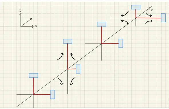
In the laboratory frame, a gravitational wave can be said to create a length change between two arbitrary points in space with the sign of . This is why the sensitivity of the advanced LIGO detectors to gravitational waves is a huge technological achievement, and the gravitational wave data are a valuable new font of information about the depths of the universe. Black hole and neutron star binary mergers are some of the most powerful events in the universe, but are completely invisible to observers on Earth except through the gravitational wave signature they produce [ 1 , 6 , 7 ].

The future of gravitational wave astronomy and astrophysics rests on the continued improvement of the sensitivity of gravitational wave detectors. By reducing detector noise, a loud signal like GW150914 can be better resolved and more accurate information can be learned from the signal. From the clearer signals, we can better resolve the physical parameters of the mergers such as masses, spins, distance, inclination of the orbital plane and sky location.

Figure 1.1: Effect of a passing linearly polarized h + gravitational wave traveling in the z direction on two test masses on the x - and y -axis

ADVANCED LIGO DETECTOR DESIGN AND O3 UPGRADES

The multiple reflections within the arm cavities increase the interaction time of the laser with the GW. The phase of the emitted light is controlled so that the quantum shot noise is minimized. The GW signal from the Advanced LIGO interferometer is amplified due to the high laser power resonating in the Fabry-Perot arms (see Section B.4).

Quantum radiation pressure noise (QRPN) is displacement noise arising from amplitude fluctuations of the electric field in the arms. The amplitude fluctuations are quantum in nature due to the quantum vacuum at the antisymmetric junction of the beam-splitting interferometer [48]. Seismic noise is the movement of the core optics due to the movement of the Earth.

Figure 2.1: Simplified diagram of the optical layout of LIGO Hanford for O3 [2].

SENSITIVITY OF THE ADVANCED LIGO INTERFEROMETERS DURING OBSERVING RUN THREE

"Locking" the detector is the process of achieving laser resonance in all parts of the interferometer at the same time, so the detector is sensitive to gravitational waves. The power of the circulating laser in the hand cavities regulates the optical gain of the interferometer's response to the gravitational wave signals. The power of the arm is difficult to accurately estimate due to the large uncertainty in the power at the beam splitter and the optical gain of the arm cavities.

The power at the Pbs beam splitter is estimated directly from the cavity collector for power recycling. The signal recycling cavity length (SRCL) is modulated, creating audio sidebands on the carrier laser in the signal recycling cavity. SRM Suspension Compliance:. compliance of the SRM, where F is the force acting on the SRM and is the mass of the SRM.

Each of the four photodetectors (TRX_A, TRX_B, TRY_A, TRY_B) will have slightly different losses (ηxa,ηxb,ηya, ηyb). However, the IMC lies in the path of the laser to clear the beam and stabilize the laser frequency. Values are those typical for LIGO Hanford during O3, locked in low noise with input power on the PRM pin = 34 W. The CARM and IMC plantsC and I include both the intrinsic optical gain of the cavity and all optical losses, incl. bundle dumps.

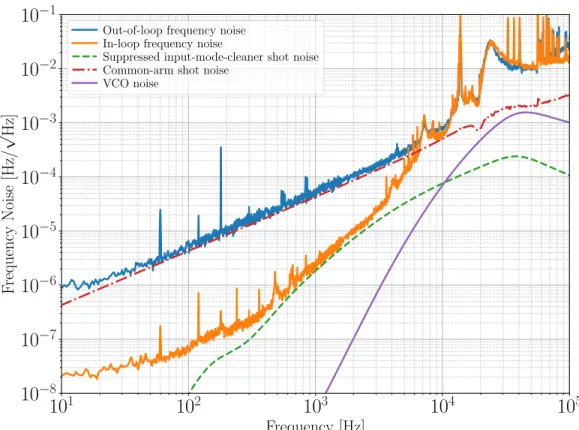
The bump at 18 kHz is due to an unmodeled resonance of the 9 MHz sidebands in the arms. The Output Mode Cleaner (OMC) is a bow tie cavity on the antisymmetric port of the interferometer. Intensity noise on the carrier will also be cleaned by the CARM and DARM coupled cavity poles of the interferometer.

This section will report on the latest understanding of the DARM facility at LIGO Hanford in O3. We modified Eq.3.57vs Ward Eq. The L factor comes from the conversion to DARM gauges because L− =hL, PLO is the local oscillator from the DARM offset beating with the GW signal on the PD, and the √ factor. 2 follows from the quadrature definition, which is evident from the difference in the prefactor between e.g. This is one likely mechanism for the effect of the SR3 disc heater on the DARM optical spring.

Figure 3.1: Differential arm noise budget for LIGO Hanford in O3 [2]. Also included are the instrument noise floors for previous observing runs, as originally presented in [43] and [92], and the Advanced LIGO design sensitivity [20].

CALIBRATION OF THE ADVANCED LIGO DETECTORS

The accuracy and precision of the models C(model) and A(model) define the systematic error and statistical uncertainty in the estimated time series h(t). This cancels the homodyne nullz with one of the DARM poles, leaving only a factor of 1+if /frse in the denominator. The first term is the explicit correction for the time dependence of the coupled cavity pool,frse(t).

The remaining components of the activation phase model, [HiAi](model)(f, ~λi), may contain systematic errors. The effect of the photon calibrator on the test mass is ultimately based on the intensity measurement via the integration sphere. Each sample response function is constructed by sampling the tails of the response function components.

Figure 4.9 shows the calibration uncertainty at the time of the most recent detection, GW170104. The extreme uncertainty refers to the maximum and minimum systematic error±1σ uncertainty within a given frequency band. This consistency is mainly due to the correction of the scale factors κT(t), κP U(t), and κC(t) in the calibration pipeline models.

The systematic error was a few percent and can be seen reflected in the upper percentiles of the Hanford uncertainty in Figure 4.10. The biggest changes in the calibration at Hanford were due to clipping of the photon calibrator laser, which misreported the strength of our response. Another advantage is that the beatnote sensor can have a relatively narrow audio bandwidth due to the length of the LIGO arms.

SL,dof(fi) is the ASD of the noise in the degree of freedom in units ofm/√.

Figure 4.1: Estimated GW150914 strain time series, i.e. waveform, produced using the PhenomD waveforms calculated via PyCBC [169, 170].

CORRELATED NOISE

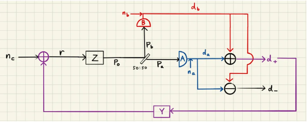
However, shot noiseshna, nai andhnb, nbi cancel out the correlated noise for most of the bandwidth. By cross-correlating hda, dbi DCPDs and removing the DARM loop, correlated noise can be eliminated. By measuring the individual DCPDda and dband signals using the DARM loop gainG and the detection function C, the correlated noise from the interferometer can be directly estimated.

For the derivation of the shot noise, we assume that the correlated noise of the GW signal and the interferometer is zero. The cross-spectral density of the shot noise is the important quantity that arises when calculating the correlated noise between DCPDs. Figure 5.5 shows the measured correlated noise with squeezing, illustrating how in the shot noise dominated frequency band the phase is 180◦.

We assume here that the correlated noise is the same for both compression and non-compression times. Above 3 kHz, the correlated noise is consistent with laser intensity noise coupling to DARM. Figures 5.4 and 5.5 plot the amplitude and phase of the correlated noise as calculated for both unsqueezing time (Eq. 5.12) and time.

This can be directly compared to the sum of the correlated noise budget traces, seen in black. Equation 5.27 shows how classical and quantum correlated noise appear in the final expression. In Figure 5.5, the measured phase of the squeezed correlated noise is shown to be 180◦ in the quantum-dominated regime.

The correlated noise budget is useful for verifying the DARM noise budget traces and determining where the classical noise is below the quantum shot noise.

Figure 5.1: Simplified DARM control loop diagram, including the two- two-photodetector sensing scheme

PROBABILITY DISTRIBUTIONS FOR SPECTRAL DENSITIES

In words, the probability that x falls between the values ofaandb is the integral of the PDF from a to b. This will motivate why the mean of PSD is a natural estimate of power i. The convolution theorem states that a Fourier transform of the convolution of two functions F(f∗g) in the time domain is equal to a multiplication in the frequency domain F(f)F(g):.

The PSD prefactor2/(N fs) changes the variance of the resulting exponential distribution, as shown in Equation 6.39. Gaussian random variables describe the real and imaginary part of the Fourier transform of Gaussian noise. Note that the characteristic function of the PDF described in Eq.6.52 is Product of Gaussian with itself and another Gaussian A(A+C) In the next section it will be important that we know the PDF of a random variable.

Therefore, the random variable V characterizing the imaginary part of CSDhx follows a Laplace distribution [207]. If we scale the distribution by 2/(N fs) from the definition of the CSD equation, 6.23, then. First, we generalize the CSD angle φ, allowing the variable in the exponent u → ucos(φ) + vsin(φ).

The validity of this assumption is examined in Appendix D. If we calculate the average of the asymmetric Laplace from Eq.6.76 with Eq.6.65, we recover In general, the distribution of the CSD hx, zi is a two-dimensional asymmetric Laplace describing the real and imaginary components of the CSD. The bias will always depend on the power ratio, but can also depend on the phase of the CSDφ, examined in Section 6.13.

Using median averaging, due to the logarithm appearing in the median expression of Eq.6.84, the final magnitude can vary from 0% to 4%, depending on the coherence of the signals. Figure 6.13 shows how coherence affects the final median CSD result for phase φ =π/4, which represents one of the largest possible deviations in the median due to phase. Figure 6.15 shows the results of several phases of the CSD evaluation process described in Section 6.15.